Chapter 4: The General Linear Model
Note
This chapter is a brief introduction to the General Linear Model (GLM), and how it is applied to fMRI data. For a more complete introduction to the GLM, see this tutorial by StatSoft.
Introduction
We now come to the General Linear Model, or GLM. With a GLM, we can use one or more regressors, or independent variables, to fit a model to some outcome measure, or dependent variable. To do this we compute numbers called beta weights, which are the relative weights assigned to each regressor to best fit the data. Any discrepancies between the model and the data are called residuals.
The symbols representing each of these terms are shown in the following equation, which can be shortened or expanded depending on the number of regressors in your model:
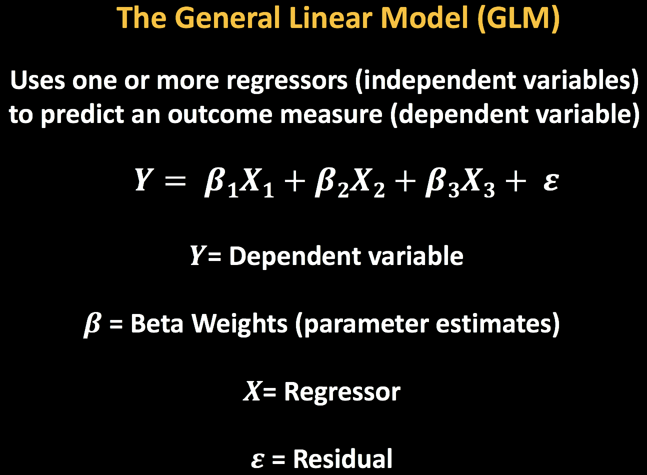
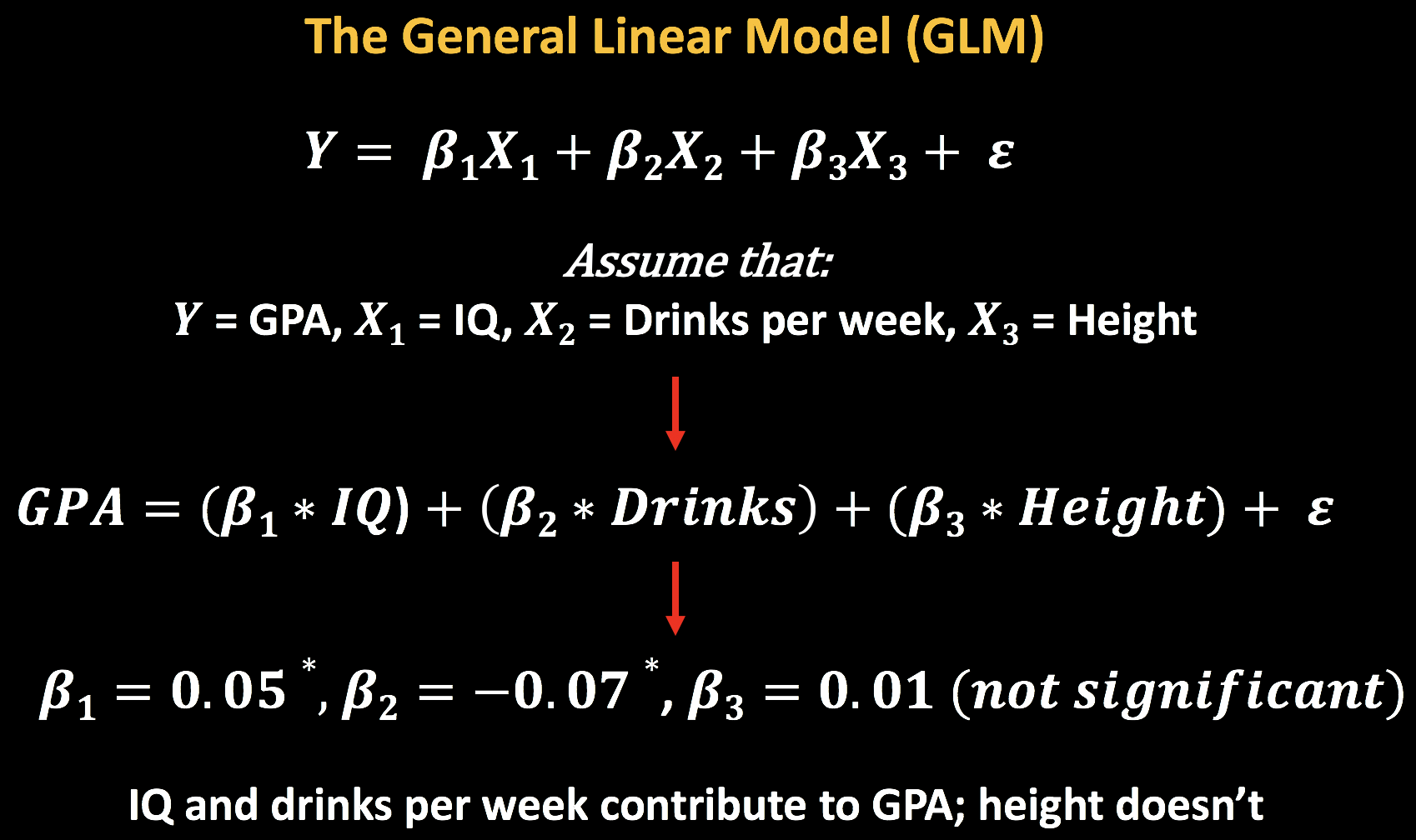
Let’s see how to apply this to a simple example. Imagine that we want to predict GPA based on height, IQ, and number of drinks per week. We may find that IQ has a positive association with GPA, number of drinks has a negative association, and height has no association at all; and we assign each of these regressors beta weights to best fit the data. For example, maybe each additional IQ point is associated with an additional 0.05 increase in GPA, while each additional drink per week is associated with a -0.07 decrease in GPA. In that case our model and its beta weights would look something like this (in which asterisks represent beta weights that are statistically significant, or are unlikely to be associated with the outome measure just by chance):
This GLM can be expanded to include many regressors, but however many there are, the GLM assumes that the data can be modeled as a linear combination of each of the regressors - hence the name General Linear Model. We will see how to apply the GLM to fMRI data in the next chapter.