fMRI Tutorial #8: 3rd-Level Analysis
Overview
Our goal in analyzing this dataset is to generalize the results to the population that the sample was drawn from. In other words, if we see changes in brain activity in our sample, can we say that these changes would likely be seen in the population as well?
To test this, we will run a 3rd-level analysis. In FSL, a 3rd-level analysis is a group-level analysis - we calculate the standard error and the mean for a contrast estimate, and then test whether the average estimate is statistically significant.
FSL can only run one model at a time. In this example, we will run a 3rd-level analysis for the contrast of Incongruent-Congruent (labeled as cope3 from the 2nd-level analysis, because it was the third contrast that was specified). As an exercise at the end of this chapter, you will be asked to run 3rd-level analyses for the individual contrast estimates of Incongruent and Congruent.
Loading the Data
From the Flanker directory, open the FEAT GUI. As with the 2nd-level analysis, select Higher-level analysis. Now, instead of selecting FEAT directories, choose Inputs are 3D cope images from FEAT directories, and change the number of inputs to 26. The 2nd-level analysis generated an average contrast of parameter estimate (or cope) for each subject for each contrast that was specified in our model. As with selecting the FEAT directories during the 2nd-level analysis, we can copy and paste a list of the cope images: Click on Select cope images and then click the Paste button. In the Terminal, navigate to the directory Flanker_2ndLevel.gfeat/cope3.feat/stats, and type ls $PWD/cope* | sort -V. This will list all of the cope images in numerical order, even though they are not zero-padded. Copy and paste the list into the Input data window by typing ctrl+y. After clicking OK, label the output directory as Flanker_Level3_inc-con.
Creating the GLM
Click on the Stats tab. For a 3rd-level analysis, we will used Mixed Effects. This models the variance so that our results are generalizable to the population our sample was drawn from. FLAME 1 (FSL’s Local Analysis of Mixed Effects) provides accurate parameter estimates by using information about both within-subject and between-subject variability; FLAME1+2 is considered even more accurate, but the additional benefit is usually minimal, and the process takes much longer.
The last option, Randomise, uses a non-parametric approach, which is valid when the assumptions about normality do not hold. Later on, we’ll discuss why this is appropriate in some cases.
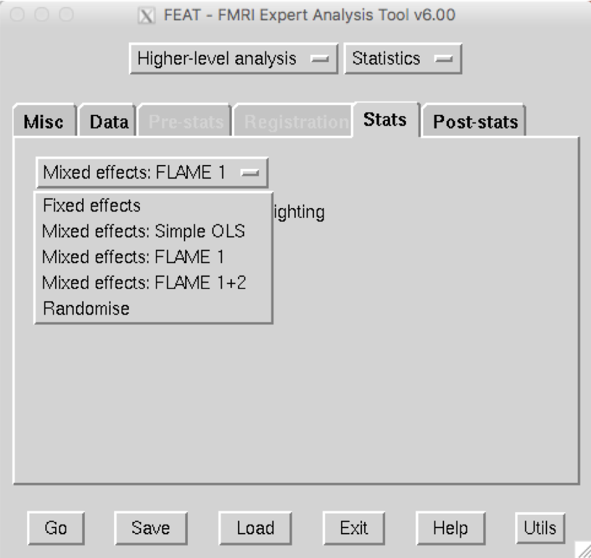
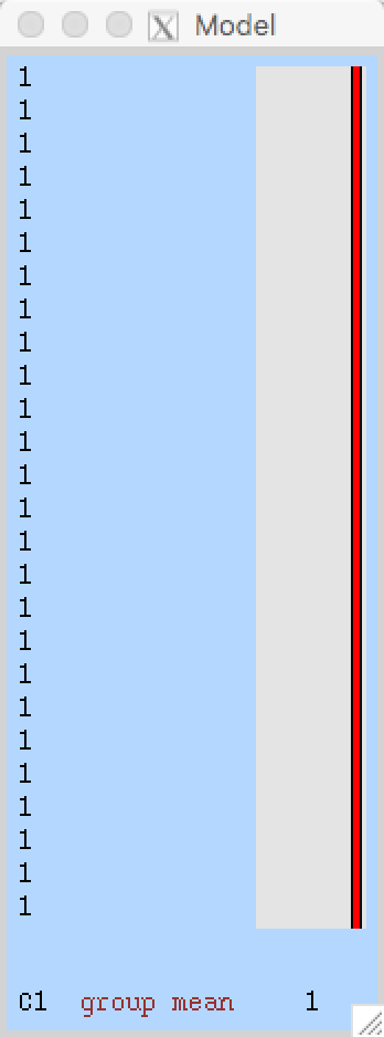
Since we’re using a simple design, we can quickly create a GLM using the Model setup wizard button. We’ve already taken the contrast for each subject, so we can select single group average. When you click Process, you should see a Model representation that looks like this:
The Post-Stats Tab
Now we finally discuss the Post-Stats tab. The only defaults you would probably want to consider changing are the Thresholding options. None won’t do any thresholding (i.e., show the parameter estimate at every voxel, regardless of significance); Uncorrected will allow any individual voxels to pass the threshold specified in Z-threshold (e.g., here we would only show voxels that have a value greater than 3.1); Voxel will perform a type of maximum height thresholding based on Gaussian Random Field theory, which is less conservative than a Bonferroni test; and lastly Cluster, which uses a cluster-defining threshold (CDT) to determine whether a cluster of voxels is significant. The logic behind this approach is that neighboring voxels are not independent of one another, and this reduced degrees of freedom is taken into account when estimating significance.
For example, if we leave our Z-threshold at 3.1 and our Cluster p-threshold at 0.05, we will look for clusters composed of voxels that each individually pass a z-threshold of 3.1. FSL runs simulations to see how often we would get clusters of certain sizes with each of their constituent voxels passing that z-threshold, and creates a distribution of cluster sizes for that CDT (similar to what happens when we compute a t-distribution based on degrees of freedom). Cluster sizes that occur less than 5% of the time in the simulations for that CDT are then determined to be significant.

For most analyses, the default of a Cluster correction analysis with a CDT of z=3.1 and a cluster threshold of p=0.05 is appropriate. For a detailed comparison of the false positive rates among the different software packages and different cluster correction settings, see the original Eklund et al. 2016 paper; for a video overview of some potential problems with cluster correction, click here.
Now click Go. This will take about 5-10 minutes, depending on how powerful your computer is.
Reviewing the Output
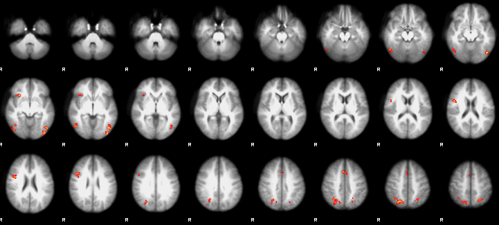
In the FEAT HTML output, you will see the thresholded z-statistic image overlaid on a template MNI brain. These are axial slices, and they give you a quick overview of where the significant clusters are located.
To take a closer look at the results, open fsleyes and load a standard template, such as MNI152_T1_1mm_brain. Then load the thresh_zstat1.nii.gz image, located in Flanker_3rdLevel_inc-con.gfeat/cope1.feat. This image only shows those clusters that were determined to be significant based on the criteria you specified in the Post-stats tab.
To make the results look cleaner, change the color scheme to “Red-Yellow”, and change the “Min.” value to 3.1. You can also click on the Gear icon and change the interpolation to make the results look smoother. Lastly, click on a cluster in the dorsal medial prefrontal cortex area, and turn the crosshairs off by clicking on the crosshairs icon. (These are all cosmetic choices, and you can change them as you like.) You can then take a snapshot of this montage with the Camera icon, and include the image as a figure in your manuscript.

The end result: an image showing the significant clusters from the analysis.
Exercises
In the
Post-statstab, set the Thresholding toNone, and re-run the analysis (changing the output directory to something that indicates that no threshold is being used). Examine the results in fsleyes. How do they compare to the cluster-corrected results?Do the same procedure in the previous exercise, this time using an
Uncorrectedthreshold. Then, repeat the procedure with aVoxelthreshold. Note any differences between these results and what you generated with the cluster-corrected results. In your own words, describe why the results are different.
Video
Click here for a demonstration of how to set up and analyze a group-level analysis in FSL.