Matlab Tutorial #2: Variables and Structures
Note
Topics covered: Variables, structures, saving
Commands used: save, clear, load
Overview of Variables and Structures
Once we create a variable or set of variables, we may want to store them for future use. For example, let’s say that we have two variables, x and y, defined using the following code:
x = 10
y = 20
If we wanted to use these later, we can save them into a .mat file using the save command:
save myVariables.mat x y
Note that the format of this command is save, followed by a .mat file, which you can call anything you want. This is followed by a list of variables that you want to store in the .mat file. If you don’t provide any variables after the .mat file, by default it will save all variables in the workspace into the .mat file.
If we want to clear the workspace of all of the currently defined variables, we can remove them using the clear command. You can remove a single variable, e.g.,
clear x
Or you can clear all of the variables in the workspace by typing clear all. Let’s say that we have created the file myVariables.mat as above, and we have cleared all of the current variables in the workspace. We can recover them by using the load command:
load myVariables.mat
Note that the variables of x and y are now present in your workspace, and you can use them in the command window as you like.
If you want to save variables into a file format that can be read as a text file, you can use the -ascii option. For example, let’s say we had two columns of numbers, representing the onset of each trial (the first column), and the duration of the trial (the second column):
Onsets = [0 2; 10 1; 16 2; 24 1]
These can be saved into a new text file:
save('Onsets.txt', 'Onsets', '-ASCII')
We will return to this concept during the chapter on scripting.
As a last exercise, create another variable, z:
z = 'fMRI'
This is a string, which we can save along with the x and y variables we created earlier:
save myVars x y z
Instead of simply using the load command, we can assign the output from load into another variable, e.g.:
Variables = load('myVars')
You will now see a new object we haven’t seen before, called a structure:
Variables =

struct with fields:

x: 10
y: 20
z: 'fMRI'
Let’s explore in more detail what a structure is.
Structures
Similar to the integers and strings we have been using so far, a structure is another data type. In this case, however, it stores other data types as well, and organizes them into containers called fields. The structure we just created, Variables, has three fields. These fields, in turn, can contain sub-fields, and those sub-fields can contain sub-fields, and so on, depending on your needs.
For example, let’s say that we have a subject, and we have that person’s name, profession, hobby, and heart rate. We could create his structure using this code:
subject.name = 'Andy';
subject.profession = 'Teacher';
subject.hobby = 'Running';
subject.Heart_rate = '60';
Similarly, we could type this all on one line to achieve the same end:
subject = struct('name', 'Andy', 'profession', 'Teacher', 'hobby', 'Running', 'Heart_rate', 60)
Let’s say that we wanted to change the name field so that it now contains two components, a First and Last name. If you try typing subject.name.first='Andy', it will throw an error. We could remove the subject structure completely by typing clear subject and starting over, or we could remove that specific field by using the rmfield command:
subject = rmfield(subject, 'name')
Note that this command takes two arguments, the name of the structure (i.e., subject), and the field we want to remove (i.e., name). The first part of this command, “subject = “, will overwrite the structure, minus the field you just removed. We can then create a new structure within the structure, a field called name with two sub-fields, First and Last:
subject.name.First = 'Andy';
subject.name.Last = 'Last';
Now when you type the variable name subject, you will see the structure name located within the current structure:
  subject =

struct with fields:

  profession: 'Teacher'
       hobby: 'Running'
  Heart_rate: 60
        name: [1×1 struct]
You can add as many fields as you want; there are no limits to how many fields the structure can contain.
The SPM.mat File and Plotting
When you begin analyzing fMRI data with SPM12, at a certain point you will generate a file called SPM.mat. These files will be generated both at the first-level per subject, or at the group-level. Let’s begin with an SPM.mat file generated at the first-level. Click here to access the Psych808 repository, and then click on the file SPM_SingleSubj.mat. This is a .mat file generated during the first-level analysis for a single subject with two runs, with each run containing 146 volumes, and with 2 conditions: Incongruent and Congruent. Then, click on the Download button to download it to your computer. Move the file to your Desktop directory by typing the following in the Matlab terminal:
movefile('~/Downloads/SPM_SingleSubj.mat', '~/Desktop')
cd ~/Desktop/
Then, load the .mat file by typing load SPM_SingleSubj.mat. There will be a new variable in the workspace called SPM, which is a 1x1 structure. From the command line, type SPM, and see the following output:
SPM =

struct with fields:

    xY: [1×1 struct]
   xBF: [1×1 struct]
 nscan: [146 146]
  Sess: [1×2 struct]
factor: []
   xGX: [1×1 struct]
    xM: [1×1 struct]
    xX: [1×1 struct]
   xVi: [1×1 struct]
 SPMid: 'SPM12: spm_spm (v7738)'
 xsDes: [1×1 struct]
   swd: '/Users/ajahn/Desktop/Flanker/sub-01/1stLevel'
  xVol: [1×1 struct]
 Vbeta: [1×6 struct]
VResMS: [1×1 struct]
    VM: [1×1 struct]
  xCon: [1×4 struct]
Many of these fields have unintelligible abbreviations, but over time you will become more familiar with them. The more decipherable ones are fields such as nscan, a vector containing the number of volumes in each run, and SPMid, which is the version of SPM that was used to analyze the data. Some of the less obvious field names are those such as xY, which contains information about the files that were loaded for the first-level analysis. For example, if you type SPM.xY.P, each row is a separate volume that was loaded into the design matrix.
Some of the fields contain structures of their own which can be indexed using numbers inside parentheses. For example, if we look within the field SPM.Sess, we see that it is a 2x1 structure, corresponding to the two runs of imaging data that were used to generate this SPM.mat file. If we just wanted to focus on the first run, we would type SPM.Sess(1). This also contains fields that are structures, such as U, which is another 2x1 structure. To access the first run of this structure, we would type SPM.Sess(1).U(1), which in turn would give us a list of fields within that structure.
Lastly, take a look at SPM.xBF: the Basis Function that was used for this analysis, which in this case was the canonical hemodynamic response function. You can see what this basis function looks like by typing:
plot(SPM.xBF.bf)
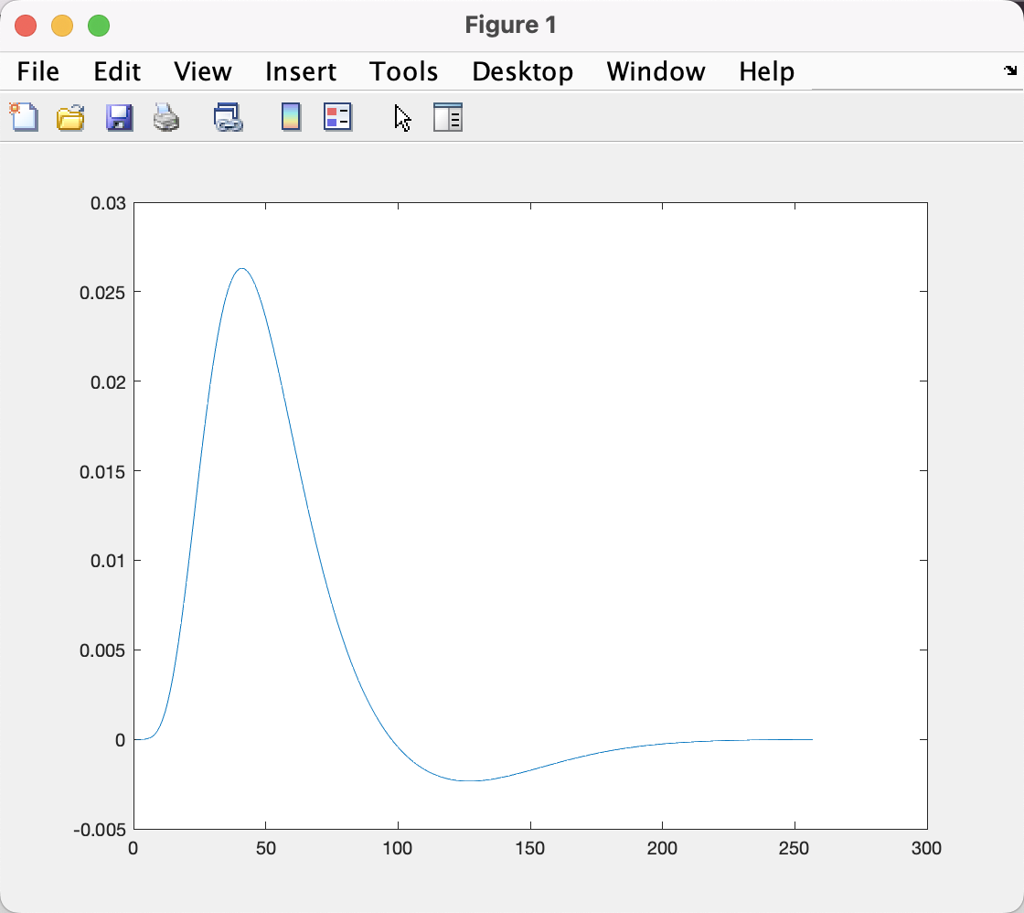
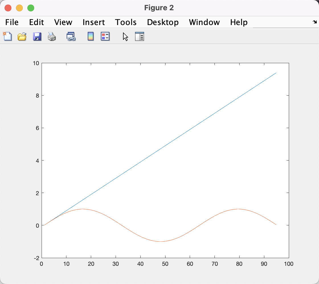
This introduces a new function, plot, which creates a 2-dimensional figure of x-values against y-values; in this example, time is on the x-axis, and the height of the BOLD response is on the y-axis. We can close the figure by simply typing close. If you want to create other plots, such as sine waves, we can define it by creating a line from 0 to 3*pi, with intervals of 0.1:
a = [0:0.1:3*pi];
figure
plot(a)

figure
plot(sin(a))
Note that the command figure precedes each plot command, and that two figures are generated as a result. If we type close, it will close the last generated figure. Alternatively, you could type close(2), using the index as an argument to close a specific figure; or, you could just type close all to close all of the figures.
If you wanted to plot two figures overlapping each other, you can use the hold command:
figure
plot(a)
hold on
plot(sin(a))
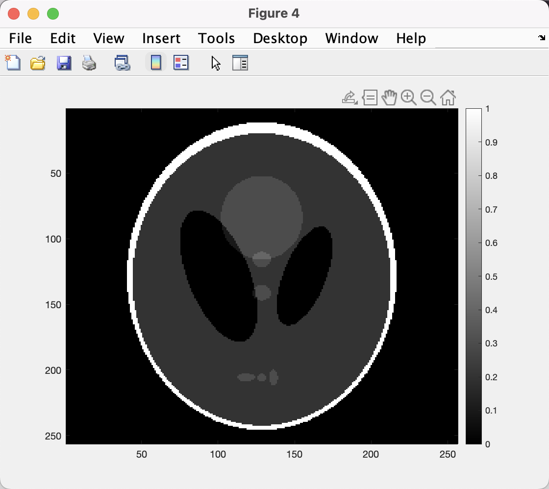
Lastly, we will plot a phantom image, or a non-living object that has been scanned using MRI. Type each of the following commands one by one, noting how the figure changes after each line of code:
figure
a = phantom;
imagesc(a)
colorbar
colormap gray
As you can see, there are many different applications of the plot command. Knowing how to use this command, and how to create and manipulate structures, will be necessary for using the more complicated .mat files generated later on by SPM.
Exercises
Once you have loaded the SPM.mat file, type
SPM.xY.P. Now, instead of printing every volume name to the terminal, extract the name of the 10th volume. (Hint: You will need to use the index syntax discussed in the previous chapter.) Show the code you used to do this.If you look at the field
SPM.xBF, you will see all of the parameters used to generate the basis function for this particular analysis. This basis function is also known as the canonical hemodynamic response function, which takes about 4-6 seconds to peak, and another 6-8 seconds to return to baseline. (This is explained in more detail in the chapters on SPM.) The fieldSPM.xBF.dtis the time interval that was used to generate this basis function, which by default is 0.125 seconds. In other words, each second encompasses eight of these time-steps (1 / 0.125 = 8). Type the following code:
figure; plot(SPM.xBF.bf(1:8:end))
And write down what you think it does, observing whether the hemodynamic response function seems smoother or more jagged (Hint: See the discussion in the previous chapter about indexing and the end keyword). Write the code you would use to plot the hemodynamic response function every three seconds. How does it compare to the previous figure you plotted? Why? Include the code you used, and screenshots of the figure you generated.
What we’ve just done in this last exercise is called resampling, which is taking a sample every nth step along a time-course to generate a new time-course. This concept can be applied to both the temporal and spatial domains, and will be used often when preprocessing fMRI data to a common time-course and a common space.
Within the field
SPM.xCon, which lists the contrasts that were created within this SPM structure, there is a field calledname. We can index each of the separate names by typingSPM.xCon(1).name,SPM.xCon(2).name, and so on. Imagine that the fourth contrast in this structure was mistakenly calledConand needs to be called something else, which can sometimes happen. Replace that contrast name by typing:
SPM.xCon(4).name = 'Neutral'
And overwrite the original SPM structure by typing:
save('SPM_updated', SPM)