Chapter 6: Running the First-Level Analysis
The Stats Tab
Navigate to the sub-08 directory, and type fsl from the command line. Open the FEAT GUI, and from the dropdown menu in the upper right of the Data tab, change “Full Analysis” to “Statistics”. This will grey out the Pre-stats and Registration tabs. You will also see a new button called “Input is a FEAT directory”. Click on the button, and select the FEAT directory run1.feat that you created in the last module. Click OK and ignore the warning about loading design information from the design.fsf file; we haven’t set up a model yet, so nothing will be overwritten.
Next, click on the Stats tab. There are many options, but we will only focus on a couple of them. Click on “Full model setup”, and change the Number of original EVs (or Explanatory Variables, FSL’s term for regressors) to 2. This will create two tabs, one for each regressor. In the EV name field for regressor 1, type “incongruent”. Click on the dropdown menu next to Basic shape, and select “Custom (3 column format)”. This reveals a field called “Filename”; click on the folder icon to select the timing file incongruent_run1.txt. Uncheck the “Add temporal derivative” button. (This is to make it easier to understand the design matrix; we will add the derivatives later.) Click on the “2” tab and repeat these steps, this time selecting the timing file “congruent_run1.txt”.
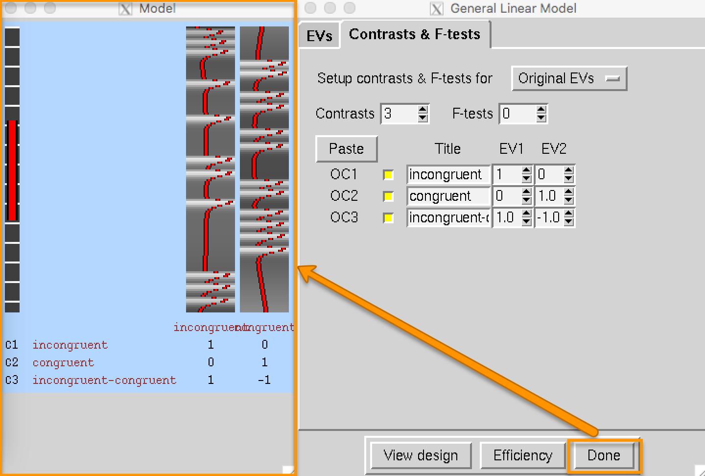
When you have finished setting up the model, click on the Contrasts & F-tests tab. This is where you specify which contrast maps you would like to create after the beta weights for each condition have been estimated. In this experiment, we are interested in three contrasts:
The average beta weight for the Incongruent condition compared to baseline;
The average beta weight for the Congruent condition compared to baseline; and
The difference of the average beta weights between the Incongruent and Congruent conditions.
Set the number of contrasts to 3, and type the following contrast names in each row, along with the following contrast weights in the EV1 and EV2 columns:
incongruent [1 0];
congruent [0 1];
incongruent-congruent [1 -1].
Note
In FSL, beta weights are called parameter estimates, or pe’s, and contrasts between beta weights are called contrast of parameter estimates, or cope’s. When we examine the output data, you will see two parameter estimate files (one for each condition), and three contrast of parameter estimate files (one for each contrast). Contrast numbers 1 and 2 above will be identical to the parameter estimate files; it may seem redundant to then recreate them, but you will see later that FSL will require the files to be labeled as cope’s for a higher-level analysis.
Click the Done button, which will open a Design Matrix window. The leftmost column represents the high-pass filter, which removes any frequencies that are longer than the length of the red bar (i.e., low frequencies are removed, and higher frequencies are allowed to pass through the filter). The two columns on the right represent the ideal time-series for both regressors, and they correspond to the order in which we entered the timing files; in other words, the first column is the ideal time-series for the Incongruent condition, and the second column is the ideal time-series for the Congruent condition.
The red line represents what we think the time-series of the voxel should look like if it is responsive to that regressor. You will notice that the white bars represent the HRF that is convolved with the onset of each trial for that condition. Take another look at the timing files for each condition and see if the correspondence between the onset times and the design matrix makes sense to you. Then, click Go to run the model.

The Post-Stats Tab
The last tab in the FEAT GUI is called Post-stats. Again, there are many options here, and the only ones you are likely to change are ones labeled “Z threshold” and “Cluster P threshold”, which are the thresholds that determine which voxels are statistically significant for each contrast. We will leave these alone for now, and come back to these options when doing a group-level analysis.
The Ideal Time-Series and the GLM
After you click Go, a series of HTML pages will open up to track the progress of the model fitting, which will take about 5-10 minutes to finish. While you’re waiting, let’s take a look at how the model we just created relates to the GLM. Remember that each voxel has a BOLD time-series (our outcome measure), which we represent with Y. We also have our two regressors, which we will represent with x1 and x2. These regressors constitute our design matrix, which we represent with a large X.
So far, all of these variables are known - Y is measured from the data, and x1 and x2 are made by convolving the HRF and the timing onsets. Since matrix algebra is used to set up the design matrix and estimate the beta weights, the orientations are turned ninety degrees: Normally we think of the time axis as going from left to right, but instead it is depicted as going from top to bottom. In other words, the onset of the run begins at the top of the timecourse.
The next part of the GLM equation is the beta weights, which we represent with B1 and B2. These represent our estimate of the amount the HRF needs to be scaled for each regressor to best match the original data in Y - hence the name “beta weights”. The last term in this equation is E, which represents the residuals, or the difference between our ideal time series model and the data after estimating the beta weights. If the model is a good fit, the residuals will decrease, and one or more of the beta weights are more likely to be statistically significant. The correspondence of the GLM to the fMRI model you created is illustrated in the animation below.

Examining the Output
When the model estimation finishes, click on the Stats link to see the design matrix. This is the same as what we just reviewed; and there is another figure below that is labeled “Covariance matrix & design efficiency”. For now, know that it is reasonable if the percentage signal changes necessary to detect each contrast are below 2%.
Click on the Post-stats link to see a thresholded map for each contrast. This shows in each contrast map any voxels that passed the significance threshold specified in the Post-stats tab of the FEAT GUI.
Exercises
Video
Click here for a demonstration of how to set up the 1st-level model for a single run.