Chapter #1: FIR Analysis in AFNI
Overview
In AFNI, the individual time-points you estimate are called TENTs - possibly because each basis function looks like a pup tent. The peak of this TENT function is estimated for each time-point that is specified, including the end-points of the interval; for example, if you wanted to estimate each time-point from zero (that is, when the stimulus occurs) to twelve seconds after the start of the stimulus, there would be seven estimates total: at the time-points 0, 2, 4, 6, 8, 10, and 12.
To begin, navigate to the directory ToneCounting_AFNI by opening a Terminal and typing cd ToneCounting_AFNI. Then, download this script to the ToneCounting_AFNI directory, and execute the script by typing bash make_AFNI_Timings_TENT.sh. This will create two separate timing files for each subject, tone_counting_onset_times.txt and tone_counting_probe_onsets.txt.
For the rest of this analysis, we will make edits to the cmd file provided on the study’s associated NITRC website (the directory can be found by clicking on the button See All Files next to the Download dropdown menu, and selecting afni_hrf_tent.tar.gz). This file uses the command afni_proc.py to create a script with all of the individual AFNI commands needed to do each step of the preprocessing and statistical analysis.
Editing the Script
To use the script in a for-loop to analyze all of the subjects in this dataset, we will change the set subj line to equal $1, so that our input from the for-loop will be the subject identification code. To save time, we will also insert the line -regress_run_clustsim no. The edited script will look like this:
#!/usr/bin/env tcsh

# created by uber_subject.py: version 0.37 (April 14, 2015)
# creation date: Tue Mar 22 11:56:09 2016

# set data directories
set top_dir = $PWD

# set subject and group identifiers
set subj      = $1
set group_id  = ToneCounting

# run afni_proc.py to create a single subject processing script
afni_proc.py -subj_id $subj                                      \
        -script proc.$subj -scr_overwrite                        \
        -blocks tshift align tlrc volreg blur mask scale regress \
        -copy_anat $top_dir/anat/${subj}_T1w.nii.gz                    \
        -tcat_remove_first_trs 0                                 \
        -dsets $top_dir/func/${subj}_task-tonecounting_bold.nii.gz     \
        -volreg_align_to third                                   \
        -volreg_align_e2a                                        \
        -volreg_tlrc_warp                                        \
        -blur_size 4.0                                           \
        -regress_stim_times                                      \
            $top_dir/func/tone_counting_onset_times.txt               \
            $top_dir/func/tone_counting_probe_onsets.txt              \
        -regress_stim_labels                                     \
            tone_counting probe                                  \
        -regress_basis_multi                                     \
            'TENT(0,12,7)' 'TENT(0,14,8)'                        \
        -regress_censor_motion 0.3                               \
        -regress_make_ideal_sum sum_ideal.1D                     \
        -regress_run_clustsim no                                \
        -html_review_style none

tcsh -xef proc.$subj |& tee output.proc.$subj
Either make these edits to the original script, or copy and paste the above code into a file called cmd.ap.AFNI_Tent. The main difference between this analysis and previous ones using the canonical hemodynamic response function is the line -regress_basis_multi 'TENT(0,12,7)' 'TENT(0,14,8)', which uses a TENT analysis for the onset_times condition spanning an interval from 0 to 12 seconds with 7 TENTs each, and 8 TENTs spanning the interval 0 to 14 seconds for the probe_onsets condition. Make sure the above script is in the folder that contains all of the subjects, and then copy and paste the following code into your terminal:
#!/bin/bash

if [[ ! -e subjList.txt ]]; then
  ls | grep ^sub- > subjList.txt
fi

for i in `cat subjList.txt`; do
  cp cmd.ap.AFNI_Tent $i;
  cd $i;
  tcsh cmd.ap.AFNI_Tent $i;
  cd ..;
done
This will create the file subjList.txt (if it doesn’t exist already), and use a for-loop to run the above cmd script for each subject. This will take a couple of hours to run.
Examining the Results
Once the preprocessing and analysis is finished, navigate to the directory sub-01/sub-01.results. Similar to the results folder from the AFNI tutorials, we see output from all of the steps; however, if we look at the output from the statistical analysis by typing 3dinfo -verb stats.sub-01+tlrc, we see the following (truncated to just the tone_counting condition):
-- At sub-brick #1 'tone_counting#0_Coef' datum type is float:       -50.34 to         60.68
-- At sub-brick #2 'tone_counting#0_Tstat' datum type is float:     -6.03381 to       4.62057
   statcode = fitt;  statpar = 68
-- At sub-brick #3 'tone_counting#1_Coef' datum type is float:     -64.2838 to       89.6593
-- At sub-brick #4 'tone_counting#1_Tstat' datum type is float:     -5.57096 to       4.79652
   statcode = fitt;  statpar = 68
-- At sub-brick #5 'tone_counting#2_Coef' datum type is float:       -119.9 to        102.47
-- At sub-brick #6 'tone_counting#2_Tstat' datum type is float:     -5.04005 to       4.87468
   statcode = fitt;  statpar = 68
-- At sub-brick #7 'tone_counting#3_Coef' datum type is float:     -132.215 to       136.358
-- At sub-brick #8 'tone_counting#3_Tstat' datum type is float:     -5.70406 to       5.24604
   statcode = fitt;  statpar = 68
-- At sub-brick #9 'tone_counting#4_Coef' datum type is float:     -100.065 to       99.7619
-- At sub-brick #10 'tone_counting#4_Tstat' datum type is float:     -5.50184 to       5.14456
   statcode = fitt;  statpar = 68
-- At sub-brick #11 'tone_counting#5_Coef' datum type is float:      -134.37 to       156.491
-- At sub-brick #12 'tone_counting#5_Tstat' datum type is float:     -5.12016 to        6.7376
   statcode = fitt;  statpar = 68
-- At sub-brick #13 'tone_counting#6_Coef' datum type is float:     -76.8142 to        77.716
-- At sub-brick #14 'tone_counting#6_Tstat' datum type is float:     -4.45098 to        4.4271
   statcode = fitt;  statpar = 68
There are 14 sub-briks total for the tone_counting condition, with 7 beta weights (i.e., those labeled “Coef”) and 7 T-statistics. In other words, we have an average beta estimate for each time-point in a 12-second window after the onset of each tone_counting condition; these beta weights can then be submitted to a group-level analysis just like the beta weights from a canonical HRF analysis.
Plotting the TENT Activity
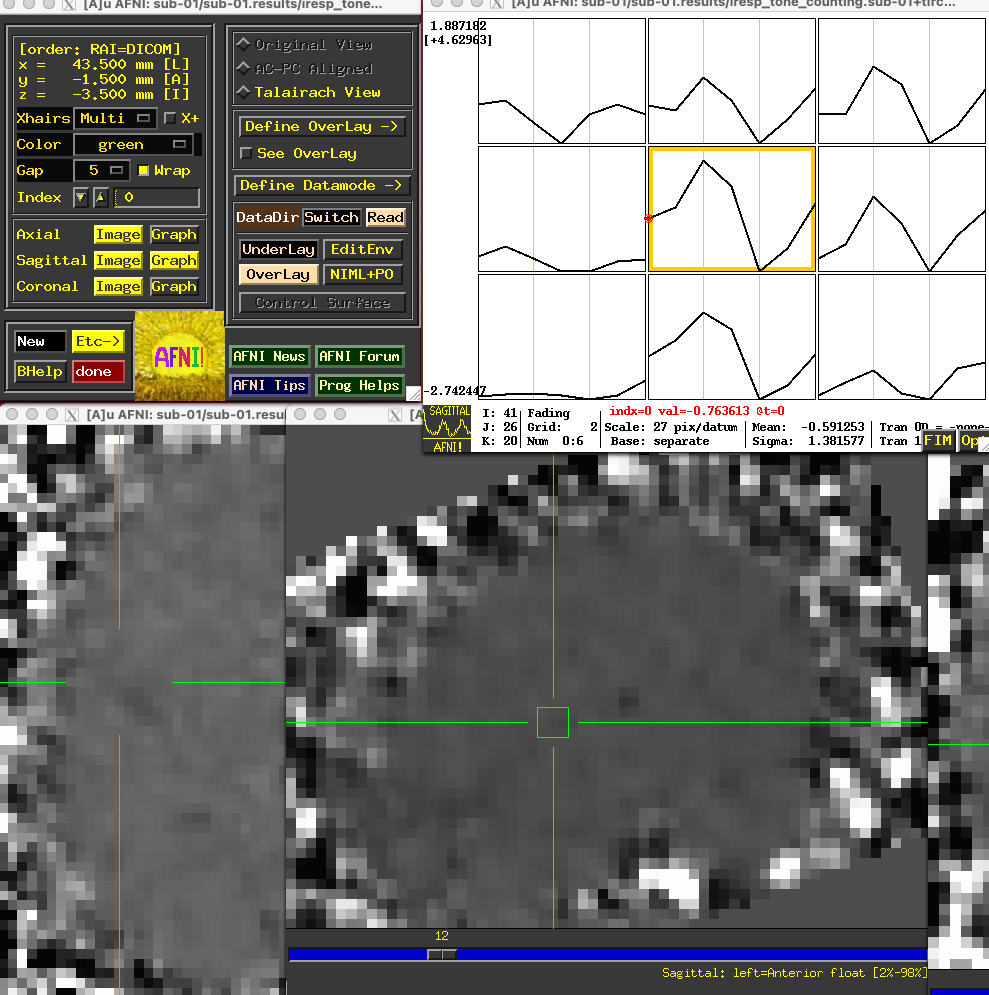
Each of the “coef” sub-briks representing the activity at each time-point are also contained within the files beginning with iresp. In this example, the file iresp_probe.sub-01+tlrc contains just the TENT sub-briks for the 14-second window after the onset of the probe stimuli, while the file iresp_tone_counting.sub-01+tlrc contains the TENT sub-briks for the tone counting stimuli. If you open the AFNI GUI by typing afni, click Underlay and select the file iresp_tone_counting.sub-01+tlrc. Place the crosshairs on a voxel around the primary auditory cortex and click the Graph button next to any of the orthogonal viewers; you will see a 3x3 matrix of the center voxel and its neighbors, with the estimated activity at each time-point.
Note
Some researchers find it more useful to force the activity of the first time-point to zero as a constant baseline for comparison with the activity of the other time-points. This can be done by changing the basis function in the above script from TENT to TENTzero. Keeping all of the other options the same, the resulting activity profile at the same voxel in the above figure would look like this:
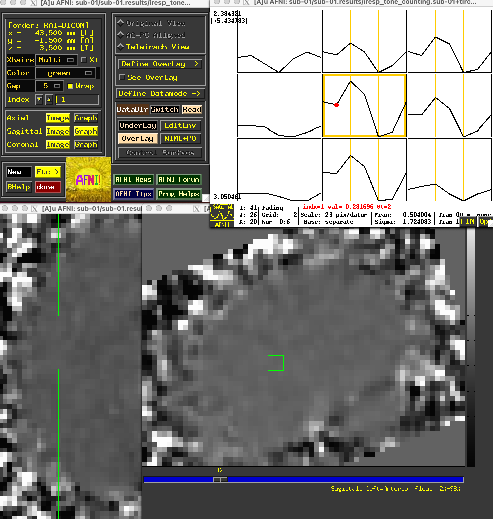
The overall profile looks almost the same, but the values are now relative to the first sub-brik’s value of zero.
Group-Level Analysis
The group-level analysis of the TENT sub-briks is virtually identical to those analyses using the canonical HRF; the only difference is that you will select which sub-briks you want to compare against each other.
For example, let’s say that we wanted to compare the zero time-point to the third time-point - in this case, those sub-briks corresponding to time-points 0s and 6s, since the TR is 2 seconds. From the above output from the stats dataset, we see that the sub-brik 7 is the third time-point after the onset of the tone counting condition, and sub-brik 1 is the onset of the condition. Thus, we could write a paired t-test script like this:
#!/bin/tcsh -xef

# created by uber_ttest.py: version 2.0 (December 28, 2017)
# creation date: Wed Feb 19 11:33:21 2020

# ---------------------- set process variables ----------------------

set mask_dset = $PWD/sub-01/sub-01.results/mask_group+tlrc

set dirA = $PWD

# specify and possibly create results directory
set results_dir = test.results_6s-0s
if ( ! -d $results_dir ) mkdir $results_dir

# ------------------------- process the data -------------------------

3dttest++ -prefix $results_dir/results_6s-0s -paired                    \
        -mask $mask_dset                                         \
        -setA SixSeconds                                           \
           01 "$dirA/sub-01/sub-01.results/stats.sub-01+tlrc[7]" \
           02 "$dirA/sub-02/sub-02.results/stats.sub-02+tlrc[7]" \
           03 "$dirA/sub-03/sub-03.results/stats.sub-03+tlrc[7]" \
           04 "$dirA/sub-04/sub-04.results/stats.sub-04+tlrc[7]" \
           05 "$dirA/sub-05/sub-05.results/stats.sub-05+tlrc[7]" \
           06 "$dirA/sub-06/sub-06.results/stats.sub-06+tlrc[7]" \
           07 "$dirA/sub-07/sub-07.results/stats.sub-07+tlrc[7]" \
           08 "$dirA/sub-08/sub-08.results/stats.sub-08+tlrc[7]" \
           09 "$dirA/sub-09/sub-09.results/stats.sub-09+tlrc[7]" \
           10 "$dirA/sub-10/sub-10.results/stats.sub-10+tlrc[7]" \
           11 "$dirA/sub-11/sub-11.results/stats.sub-11+tlrc[7]" \
           12 "$dirA/sub-12/sub-12.results/stats.sub-12+tlrc[7]" \
           13 "$dirA/sub-13/sub-13.results/stats.sub-13+tlrc[7]" \
           14 "$dirA/sub-14/sub-14.results/stats.sub-14+tlrc[7]" \
        -setB ZeroSeconds                                           \
           01 "$dirA/sub-01/sub-01.results/stats.sub-01+tlrc[1]" \
           02 "$dirA/sub-02/sub-02.results/stats.sub-02+tlrc[1]" \
           03 "$dirA/sub-03/sub-03.results/stats.sub-03+tlrc[1]" \
           04 "$dirA/sub-04/sub-04.results/stats.sub-04+tlrc[1]" \
           05 "$dirA/sub-05/sub-05.results/stats.sub-05+tlrc[1]" \
           06 "$dirA/sub-06/sub-06.results/stats.sub-06+tlrc[1]" \
           07 "$dirA/sub-07/sub-07.results/stats.sub-07+tlrc[1]" \
           08 "$dirA/sub-08/sub-08.results/stats.sub-08+tlrc[1]" \
           09 "$dirA/sub-09/sub-09.results/stats.sub-09+tlrc[1]" \
           10 "$dirA/sub-10/sub-10.results/stats.sub-10+tlrc[1]" \
           11 "$dirA/sub-11/sub-11.results/stats.sub-11+tlrc[1]" \
           12 "$dirA/sub-12/sub-12.results/stats.sub-12+tlrc[1]" \
           13 "$dirA/sub-13/sub-13.results/stats.sub-13+tlrc[1]" \
           14 "$dirA/sub-14/sub-14.results/stats.sub-14+tlrc[1]"
Visualizing these results and determining a significance threshold for them is the same as in the previous AFNI tutorials.
Note
For more details on how to set up contrasts within AFNI for to compare different TENTs, as well as a comparison of TENT to other basis functions, see this post by Pete Molfese.
Exercises
Imagine that instead of analyzing the interval of 0-12 seconds, we wanted to just look the interval of 0-8 seconds for the
tone_countingcondition. Show how you would modify theafni_proc.pyscript above, and run the script forsub-01. How has the 0-8 second interval changed compared to the previous TENT analysis, if at all? Choose a voxel located at MNI coordinates [47, 3, -6] to illustrate the comparison between the analyses.FIR analyses can also analyze an interval with a given number of TENT functions that is not divisible by your TR. For example, change the
afni_proc.pyscript for thetone_countingcondition to ‘TENT(0,12,5)’, which will span the 12-second range with 5 TENT functions; these will be interpolated to match the time grid. (Using TENTs that evenly divide into your TRs will be more accurate, but there may be theoretical reasons for using a different time scale.) Run this updated analyses, and examine how the output compares to the original afni_proc.py script, again using MNI coordinates [47, 3, -6] to illustrate the comparison between the analyses.
Video
For a video overview of how to do FIR analysis in AFNI, click here.
Next Steps
Now that you are familiar with how to analyze the data with AFNI, we will move on to analyzing the data in SPM. To see how to do that, click the Next button.