Chapter #3: FIR Analysis in FSL
Overview
Finite Impulse Response analysis in FSL is more similar to SPM than to AFNI; the basic setup happens in the GUI, and you specify a window along with the number of time-points you want to estimate. Since both the preprocessing and modeling happens within the same FEAT GUI, the analysis will be more compact than in SPM.
Before you begin, create the onset time files by navigating to the directory containing all of your subject, and then copying and pasting the following code:
#!/bin/bash

#Check whether the file subjList.txt exists; if not, create it
if [ ! -f subjList.txt ]; then
        ls -d sub-?? > subjList.txt
fi

#Loop over all subjects and format timing files into FSL format
for subj in `cat subjList.txt` ; do
        cd $subj/func #Navigate to the subject's func directory, which contains the timing files

        cat ${subj}_task-tonecounting_events.tsv | awk '{if (NR!=1 && $5=="") {print $1, $2, "1"}}' > toneCount_run1.txt
        cat ${subj}_task-tonecounting_events.tsv | awk '{if ($5=="probe") {print $1, $2, "1"}}' > toneProbe_run1.txt

        cd ../..
done
This will create new files in the func directory called toneCount_run1.txt and toneProbe_run1.txt, respectively.
Preprocessing and the First-Level Model
Now, navigate to the folder sub-01 and type Feat_gui. This will open the FEAT GUI; make sure the defaults of First-level analysis and Full Analysis are selected, and then click on the button Select 4D data. Select the file func/sub-01_task-tonecounting_bold.nii.gz, and click OK. In the field next to Output directory type run1, and leave the other defaults in the Data and Pre-stats tabs as they are. In the Registration tab, set the search values in both the Main structural image and Standard space fields to Full Search and 12 DOF (you may use BBR if you want; to make the analysis quicker, we will use these other settings). In the Main structural image field, select the image anat/sub-01_T1w_brain.nii.gz. Then, click on the Stats tab and click the button Full model setup.
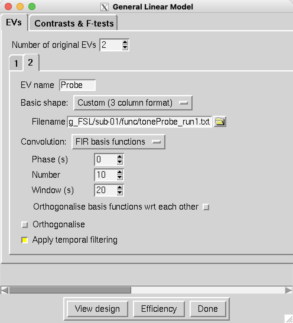
Set the Number of original EVs to 2, and for the EV name for the first regressor, type ToneCounting. Change the Basic shape to Custom (3 column format), and select the file toneCount_run1.txt. In the dropdown menu next to Convolution, select FIR basis functions. As with AFNI and SPM, you can select the time window and the number of time-points to estimate; change the Number to 10 and the Window to 20. This will estimate 10 time-points at 2 second intervals in a 20-second window after the onset of the stimulus. Click on the 2 tab to select the second regressor, give it the name Probe, and select Custom (3 column format) and the file toneProbe_run1.txt; use the same Number and Window values of 10 and 20:
Specifying the Contrasts
If you click on the Contrasts & F-tests tab, you may get a message telling you to use Real EVs; this is because the Original EVs are usually restricted to estimating the amplitude of the regressor, and ignore additional regressors such as temporal derivatives and motion regressors. In this case we are interested in the additional regressors, specifically the estimated time-points after the onset of the condition.
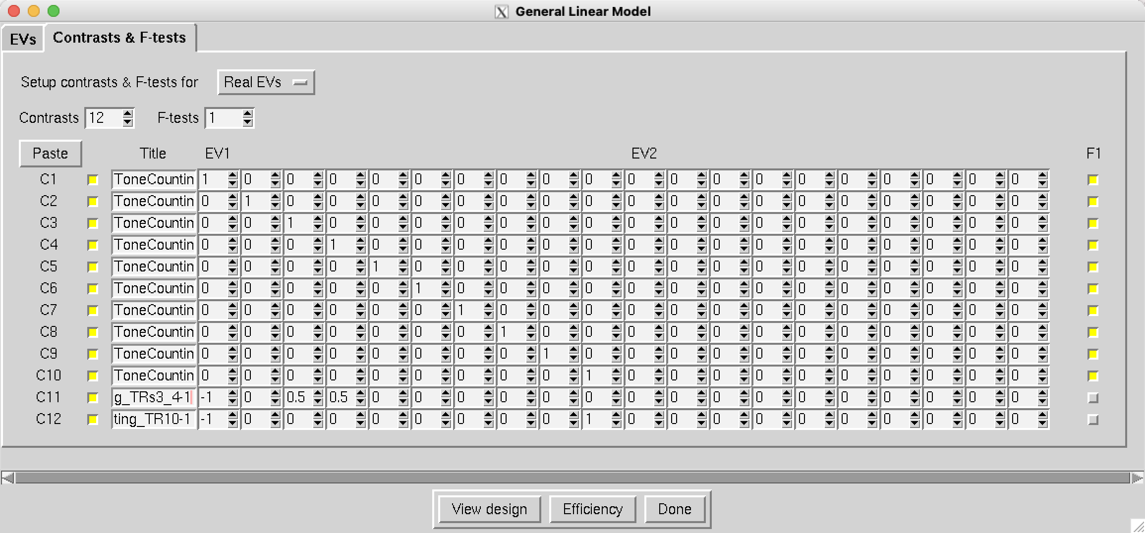
In the field next to F-tests, type 1 and press enter. You should see 10 contrasts automatically filled in with a diagonal of 1’s for each time-point after the ToneCounting condition, and a box selected in the column F1. Just as in the SPM tutorial, this will test whether there is any significant difference anywhere for any of the time-points. We can also add two more contrasts by changing the Contrasts number to 12; name these additional contrasts ToneCounting_TRs3_4-1 and ToneCounting_TR10-1, and give them the contrasts [-1 0 0.5 0.5 0 0 0 0 0 0] and [-1 0 0 0 0 0 0 0 0 1], respectively. The first will test whether the average of TRs 3 and 4 is greater than 1, and the second will test whether TR 10’s activiy is greater than TR 1’s.
Note
The box to the left of each regressor marked C1, C2, etc., will also create a separate t-contrast for that particular regressor. If you don’t want individual t-tests for each regressor, uncheck the boxes from C1 to C10, and leave the F-test boxes checked. However, these individual t-tests will be useful later on if you want to extract contrast estimates for each time-point in a group-level ROI analysis.
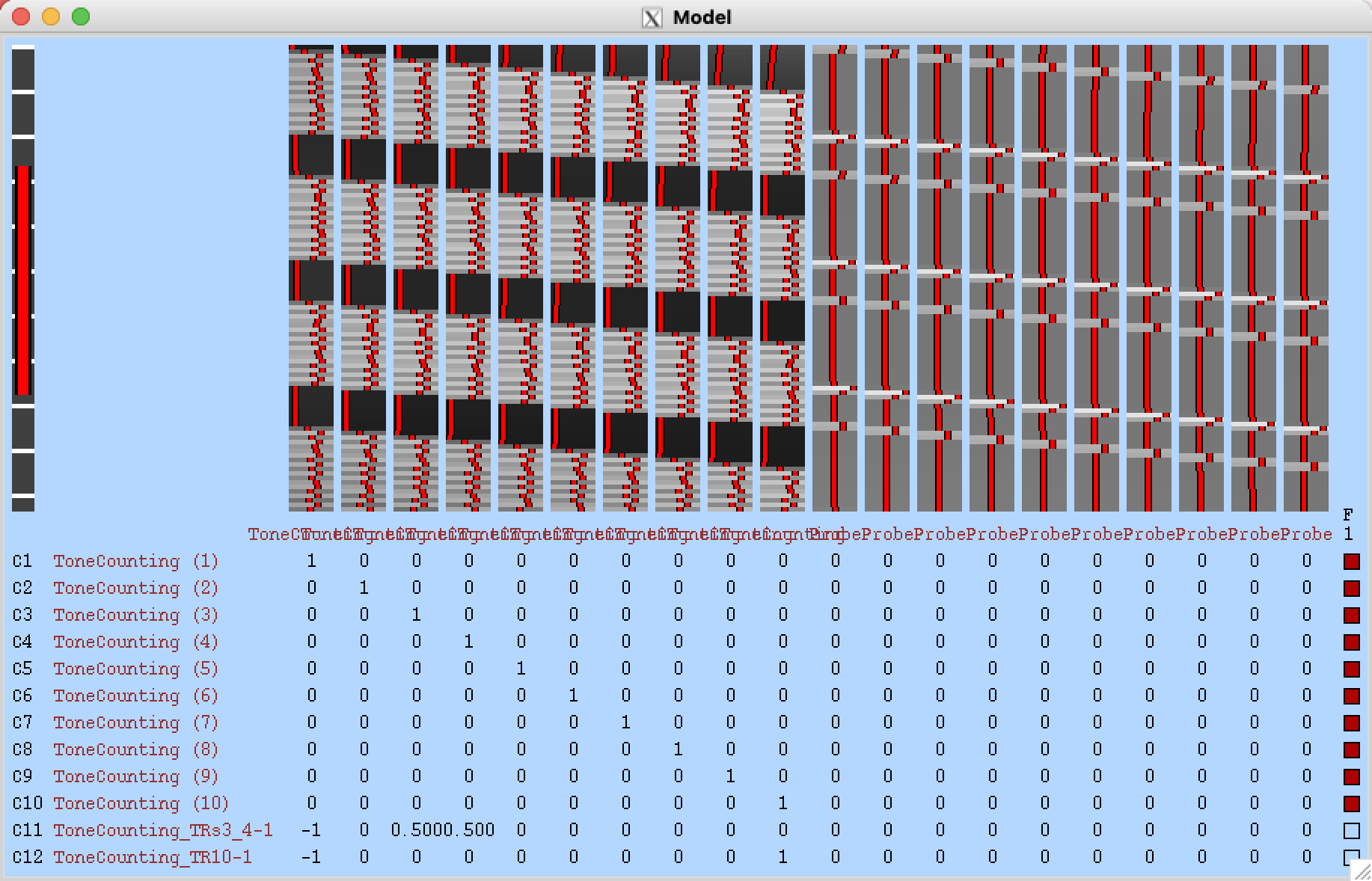
If you click on View Design, you should see the following image, representing 10 regressors after the onset of each condition:
Creating the Script
Next, click Done, and then click Save; call the output file Design_run1, and save it to the directory containing all of your subjects. Then use your terminal to navigate to the directory containing the subjects, and copy and paste the following code:
#!/bin/bash

# Generate the subject list to make modifying this script
# to run just a subset of subjects easier.

for id in `seq -w 1 2` ; do
    subj="sub-$id"
    echo "===> Starting processing of $subj"
    echo
    cd $subj

        # If the brain mask doesn’t exist, create it
        if [ ! -f anat/${subj}_T1w_brain_f02.nii.gz ]; then
            echo "Skull-stripped brain not found, using bet with a fractional intensity threshold of 0.5"
            # Note: This fractional intensity appears to work well for most of the subjects in the
            # Flanker dataset. You may want to change it if you modify this script for your own study.
            bet2 anat/${subj}_T1w.nii.gz \
                anat/${subj}_T1w_brain.nii.gz
        fi

        # Copy the design files into the subject directory, and then
        # change “sub-01” to the current subject number
        cp ../design_run1.fsf .

        # Note that we are using the | character to delimit the patterns
        # instead of the usual / character because there are / characters
        # in the pattern.
        sed -i '' "s|sub-01|${subj}|g" \
            design_run1.fsf

        # Now everything is set up to run feat
        echo "===> Starting feat for run 1"
        feat design_run1.fsf
                echo

    # Go back to the directory containing all of the subjects, and repeat the loop
    cd ..
done

echo
This will analyze all of the subjects with the FIR model you specified in the FEAT GUI; it will take a couple of hours, depending on the speed of your computer.
Note
Subjects 1 and 2 have 104 TRs in their ToneCounting runs, while subjects 4-14 have 112; subject 3 has 113. To make the script run without errors for the rest of the subjects, you will need to edit the design_run1.fsf script and change line 39 from set fmri(npts) 104` to 113 for subject 3, and 112 for subjects 4-14. Then rerun the script above, changing seq -w 1 2 to seq -w 3 for subject 3, and seq -w 4 14 for the rest of the subjects.
Viewing the FIRs
In order to view the estimated time-points as a time-series, you will need to concatenate them using fslmerge. Navigate to the directory sub-01/run1.feat/stats and type the following:
fslmerge -t FIRs.nii.gz zstat1.nii.gz zstat2.nii.gz zstat3.nii.gz zstat4.nii.gz zstat5.nii.gz zstat6.nii.gz zstat7.nii.gz zstat8.nii.gz zstat9.nii.gz zstat10.nii.gz
This will create a new file, FIRs.nii.gz, which you can look at in fsleyes. Type fsleyes from the command line to open up the viewer, and then select File -> Add from file, and choose the file sub-01/run1.feat/reg/highres.nii.gz. Then select File -> Add from file, navigate to the sub-01/run1.feat/stats directory, and select the file fstat1.nii.gz and FIRs.nii.gz. Highlight the fstat1 file, threshold it however you want, and note where there seem to be brighter intensity voxels, indicating a higher f-statistic. Then highlight the FIRs file, and click on View -> Time Series. You should see something like this:
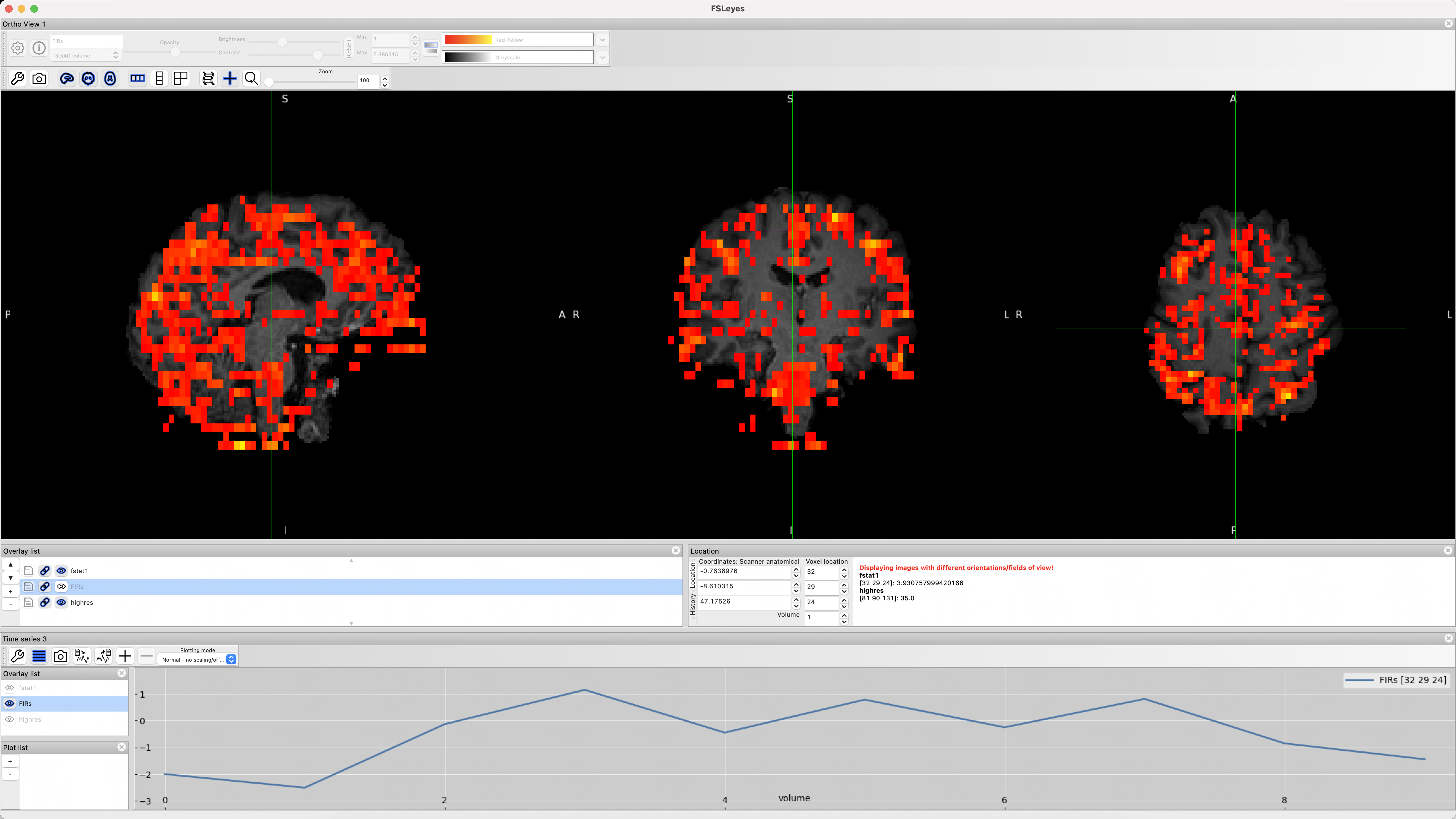
As you click the crosshairs on different voxels, the time-series will update to show the estimated BOLD response to each time-point in the window you specified. Once you run the preprocessing and first-level analysis for all of the subjects, you can then do a group-level analysis on the time-points and contrast that you want, and extract time-points using an ROI analysis as in the Flanker study.
Video
For a video demonstration of how to do FIR analysis in FSL, click here.
Next Steps
You have now learned how to perform a Finite Impulse Response analysis in all of the major software packages; which one you choose is ultimately up to you.