FreeSurfer Tutorial #9: Cluster Correction
Overview
After you have run your general linear model and created group-level contrast maps, you will need to correct for the amount of tests that you have run. For a more detailed overview of how cluster-correction works, see this page. Although it uses fMRI data to illustrate the concept, the same idea applies to the vertices that we analyze in structural data.
Cluster Correction with mri_glmfit-sim
As in the previous tutorial, we will use nested for-loops to create cluster-corrected maps for each contrast. Each level of the nested loop specifies a different combination of which hemisphere, smoothness, and structural measurement we are analyzing:
#!/bin/tcsh

setenv study $argv[1]

foreach meas (thickness volume)
  foreach hemi (lh rh)
    foreach smoothness (10)
      foreach dir ({$hemi}.{$meas}.{$study}.{$smoothness}.glmdir)
        mri_glmfit-sim \
          --glmdir {$dir} \
          --cache 1.3 pos \
          --cwp 0.05  \
          --2spaces
      end
    end
  end
end
The options for mri_glmfit_sim specify the following:
The directory that is being corrected for multiple comparisons (
--glmdir);The vertex-wise cluster threshold (
--cache);The cluster-wise p-threshold (
--cwp, always set to 0.05 unless you have reasons for doing otherwise);Correction for analyzing both hemispheres (
--2spaces)
For most analyses, the --glmdir, --cwp, and --2spaces options will not need to be changed. The --cache option, on the other hand, may be changed depending on your analysis; and so it deserves to be explained in more detail.
The first argument to the --cache option is the vertex-wise threshold - only vertices above this threshold will be considered part of the clusters that will then be tested for statistical significance. The following table shows you which vertex-wise thresholds have been cached, or already stored in memory. (These were generated by using the --qcache option during recon-all.) In other words, FreeSurfer has pre-computed the number of contiguous vertices at each vertex-wise threshold in order to be labeled a significant cluster. The following cluster-defining thresholds are available for use with the mri_glmfit-sim command as the first argument after the -cache option; you can choose any of the -log10(P) values in the lefthand column, which correspond to the p-values in the righthand column:
-log10(P) value |
p-value |
|---|---|
1.3 |
0.05 |
2.0 |
0.01 |
2.3 |
0.005 |
3.0 |
0.001 |
3.3 |
0.0005 |
4.0 |
0.0001 |
The second argument after the --cache option specifies the direction of the test you are analyzing: The positive direction (pos), the negative direction (neg), or both directions (abs). If you have an a priori hypothesis about which group should have larger or smaller structural values, use the pos or neg arguments; otherwise, use the abs argument.
Warning
If you are using the --cache option, it is now recommended to use a value of 3.0 or higher. A recent paper by Greve & Fischl (2018) demonstrated that using a lower vertex-wise threshold leads to inflated false positives. To maintain a false positive rate of 0.05, either use a vertex-wise threshold of 3.0, or use a permutation test with the --perm option. See the help output of mri_glmfit-sim for more details.
Now copy the code above into a file called runClustSims.sh, and save it in the directory containing your subjects. (A copy of the above script is available here.) You can run the script by typing runClustSims.sh CannabisStudy.
Viewing the Results
When the script has finished, navigate into one of the directories that it has analyzed, such as lh.volume.CannabisStudy.10.glmdir/HC-CB. There are several new files that have been created:
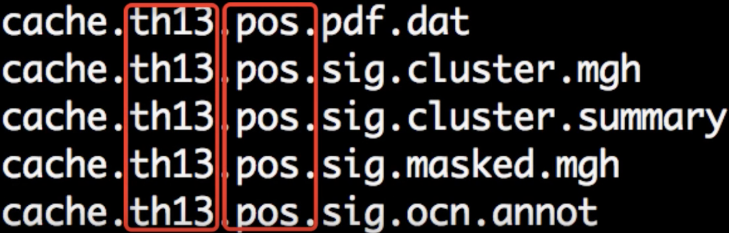
Each part of the filename is separated by periods. The first part, cache indicates that the cluster simulation was performed using cached simulations; th13 means that a vertex-wise threshold of 1.3 was used; and pos indicates the direction of the test.
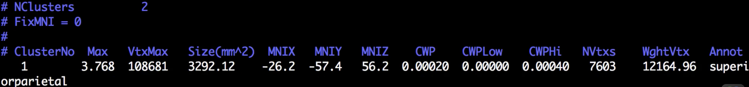
Although there are many files that have been generated, we will focus on only two of them: The cluster.summary and cluster.mgh files. If you open the cluser-summary file and scroll to the bottom, you will see a listing of each cluster that was determined to be statistically significant:
These clusters can then be rendered on the fsaverage template by typing the following from the cluster-corrected directory:
freeview -f $SUBJECTS_DIR/fsaverage/surf/lh.inflated:overlay=cache.th13.pos.sig.cluster.mgh
Observe how the clusters that you see in freeview correspond to the clusters listed in the cluster summary file.
Summary
This concludes how to run structural analyses between groups; you can use the above code as templates for analyzing the groups in your study. For many experiments, this will be all the researcher needs.
Even if your main focus is testing for group differences, however, you might want to do other supplementary analyses - such as correlation analyses and region of interest analyses. We will cover those in the next two chapters.
Video
For a video overview of how to do cluster correction in FreeSurfer, click here.