FreeSurfer Tutorial #11: Region of Interest Analysis
Overview
In addition to creating a cortical surface and calculating structural measurements at each vertex, FreeSurfer parcellates and segments the brain - the parcellations outlining anatomically distinct regions of the cortex, and the segmentations dividing the sub-cortical nuclei into distinct structures. These parcellations are created along the lines of two atlases that come with FreeSurfer: The Destrieux atlas, and the Desikan-Killiany atlas.
Within each subject’s stats directory, there is a table corresponding to the parcellations for each atlas. For example, the results for the parcellation of the left hemisphere are located in the file lh.aparc.annot for the Desikan-Killiany atlas, and in the file lh.aparc.a2009s.annot for the Destrieux atlas. The main difference between the two is that the Destrieux atlas contains more parcellations which can be used for finer-grained analyses.
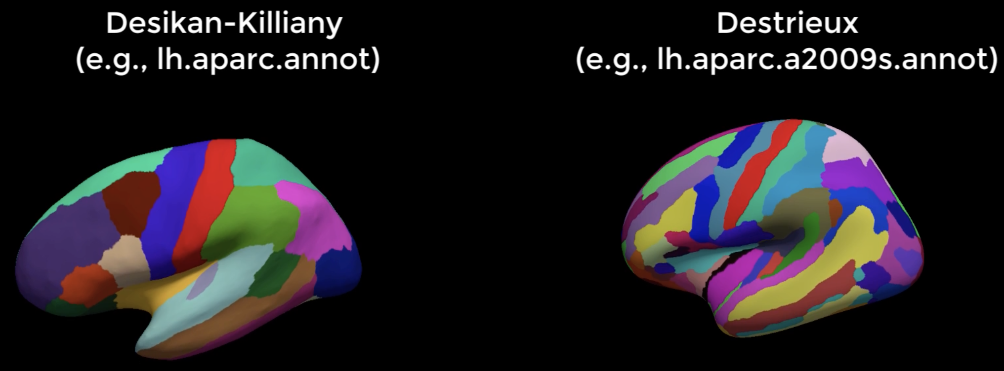
The Desikan-Killiany and Destrieux atlases placed side by side. Note that the Destrieux atlas contains more parcellations of the cortex.
The segmentations, on the other hand, are contained within one file called aseg.stats. There are no separate segmentation files for each atlas.
Extracting data with asegstats2table and aparcstats2table
Both the command asegstats2table and aparcstats2table require a list of subjects and the structural measurement you wish to extract from the table.
Let’s begin with asegstats2table. A typical command would look like this:
asegstats2table --subjects sub-101 sub-103 --common-segs --meas volume --stats=aseg.stats --table=segstats.txt
The
--subjectsoption specifies a list of subject names;--common-segssignalizes to output segmentations common to all of the subjects - in other words, if one subject’s number of segmentations is different from the others, do not exit the command with errors;--measindicates which structural measurement to extract from the table (“volume” is the default; alternatives are “mean” and “std”);--statspoints to the stats file that the segmentation data will be extracted from; and--tablewrites the extracted measurement to a text file, organized by subject name.
The command aparcstats2table requires similar arguments. Here is a typical command:
aparcstats2table --subjects sub-101 sub-103 --hemi lh --meas thickness --parc=aparc --tablefile=aparc.txt
In this command you can specify the hemisphere to analyze (--hemi), the measurement to extract (--meas, with the options of “thickness”, “volume”, “area”, and “meancurv”), and which atlas to use for parcellation (--parc; you can specify either “aparc”, the Desikan-Killinay atlas, or “aparc.a2009s”, the Destrieux atlas). The label for the output file is specified with the --tablefile option. Include as many subjects as you like in your analysis.
Next Steps
The output from these commands are tab-delimited text files that can be read into a spreadsheet like Excel, or a statistical software program such as R. You would perform the statistical tests just like you would any other t-test: Select the structural measurements from the groups you wish to compare, and then contrast the two groups against each other.
Note
In the future, I will add sections on how to resample a volumetric ROI to the surface, and then extract structural measurements from that ROI. The code below was created some time ago, but it should work for most purposes.
#!/bin/tcsh

setenv SUBJECTS_DIR `pwd`

#Create 5mm sphere ROI with 3dUndump; ROI_file.txt contains x-, y-, and z-coordinates for center of sphere (e.g., 0 30 20)
3dUndump -srad 5 -prefix S2.nii -master MNI_caez*+tlrc.HEAD -orient LPI -xyz ROI_file.txt

#View in tkmedit
tkmedit -f MNI_caez_N27.nii -overlay S2.nii -fthresh 0.5

#Register anatomical template to fsaverage (FreeSurfer template)
fslregister --s fsaverage --mov MNI_caez_N27.nii --reg tmp.dat

#View ROI on fsaverage
tkmedit fsaverage T1.mgz -overlay S2.nii -overlay-reg tmp.dat -fthresh 0.5 -surface lh.white -aux-surface rh.white


#Map ROI to fsaverage surface
mri_vol2surf --mov S2.nii \
        --reg tmp.dat \
        --projdist-max 0 1 0.1 \
        --interp nearest \
        --hemi lh \
        --out lh.fsaverage.S2.mgh \
        --noreshape

#Check how well the ROI maps onto the inflated surface
tksurfer fsaverage lh inflated -overlay lh.fsaverage.S2.mgh -fthresh 0.5
Conversely, you may want to resample a surface ROI to a volume, and then extract data from it; for example, let’s say that we want to convert the superior temporal ROI created by FreeSurfer, to the individual subject’s volumetric space. First, create a registration file called register.dat with FreeSurfer’s tkregister2 command:
tkregister2 --mov beta_0001.nii --s subject --noedit --regheader --reg register.dat
Where “beta_0001.nii” is a beta map created in the subject’s native space, and “subject” is the name of the subject that has been preprocessed with recon-all.
We then use the command mri_label2vol to convert the surface ROI to volumetric space:
mri_label2vol --label lh.superiortemporal.label --temp beta_0001.nii --subject subject --hemi lh --fillthresh .9 --proj frac 0 1 .1 --reg register.dat --o $PWD/stgnew.nii
In this case, we create a new file, stgnew.nii, which is the surface ROI converted to volumetric space.
Video
For a video overview of how to do region of interest analysis in FreeSurfer, click here.