MRIcroGL Tutorial #3: Viewing Images
Overview
The main feature of MRIcroGL is the ability to view medical images - especially magnetic resonance imaging (MRI) data. For this tutorial, we will focus on MRI and fMRI, although many other forms of imaging data can be loaded as well.
In the first chapter of this walkthrough, you experimented with the basic operations of the viewer, such as the Opacity slider, the crosshairs, and the Brightness settings. We will examine these in more detail, and begin to use multiple images at once, in order to explore the abilities of the software package.
Note
Many of the steps and examples in this tutorial are taken from Chris Rorden’s MRIcroGL video, which can be found here. He covers many different types of images that can be loaded, including animal brains, spinal cords, and lungs. Here we will be focusing on MRI and fMRI data, but I encourage you to look at the other images in your own time.
This tutorial also assumes that you have completed the analysis of the Flanker dataset in any of the major fMRI analysis software packages - SPM, FSL, and AFNI. Here we will be using the fully preprocessed and statistically analyzed data using FSL, but the parallels with the outputs of any of the other packages should be clear.
Loading a Functional Image
We will begin by loading a functional image - in this case, the T2*-weighted sub-10_T1w image from sub-10/func folder in the Flanker directory. You will see something like this:
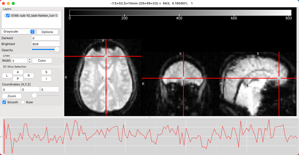
As you saw in an earlier chapter, left-clicking and dragging in any of the window panes will move the crosshairs, which in turn updates the view in the other two panes. You can keep the crosshair where it is and scroll through the slices in the current pane by scrolling the mouse wheel either up or down; holding the ctrl key while scrolling allows you to zoom in and out of the image. Scrolling one image at a time can be done manually by clicking on the L, R, A, P, S, and I buttons in the 2D Slice Selection subwindow. If you prefer a different color for the crosshair, click the Color button and select any color that you like. The width of the crosshairs can also be modified by increasing or decreasing the value in the Width field.
Note
A full list of the combination of mouse clicks and button presses can be found by clicking on Help -> Mouse Gestures.
You will also see a time-series displayed at the bottom of the viewing window, representing the signal intensity for the voxel at the center of the crosshair. Clicking at a different part of the time-series will jump to that volume, and the volume index will be updated in the Layers window. For example, 55/146 means that you are currently viewing the 55th volume in the time-series, out of 146 volumes total. You can flip through the volumes by either pressing option+N to advance one volume or option+V to go back one volume, or flip through the volumes automatically at a steady rate by clicking Display -> Animate Volumes. Similar to FSLeyes, you can also generate a seed-based correlation map by selecting Display -> Seed Correlation (Pearson). This will create a correlation map displaying the connectivity between the time-series centered at your crosshairs, and every other voxel in the brain.
Loading an Anatomical Image
Next, we will load an anatomical image - in this case, the T1-weighted sub-10_T1w image from sub-10/anat folder in the Flanker directory. You will see something like this:
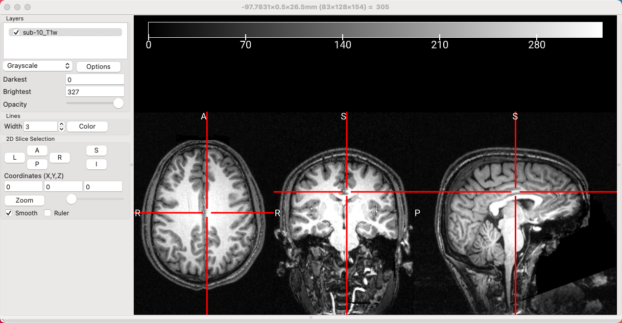
An anatomical image. Note that this image has had the face removed, in order to deidentify it.
Modifying the values in the Darkest and Brightest fields are useful for setting the thresholds for which voxels will be shown. For example, you may not want to see any voxels below an intensity of 30, for example, or anything brighter than an intensity of 300. By setting the Darkest threshold to 30 and the Brightest threshold of 300, the darkest color - in this case, black - will be set to those voxels with an intensity of 30, and white will be assigned to those voxels with an intensity of 300.
Viewing the Intensity over Slices
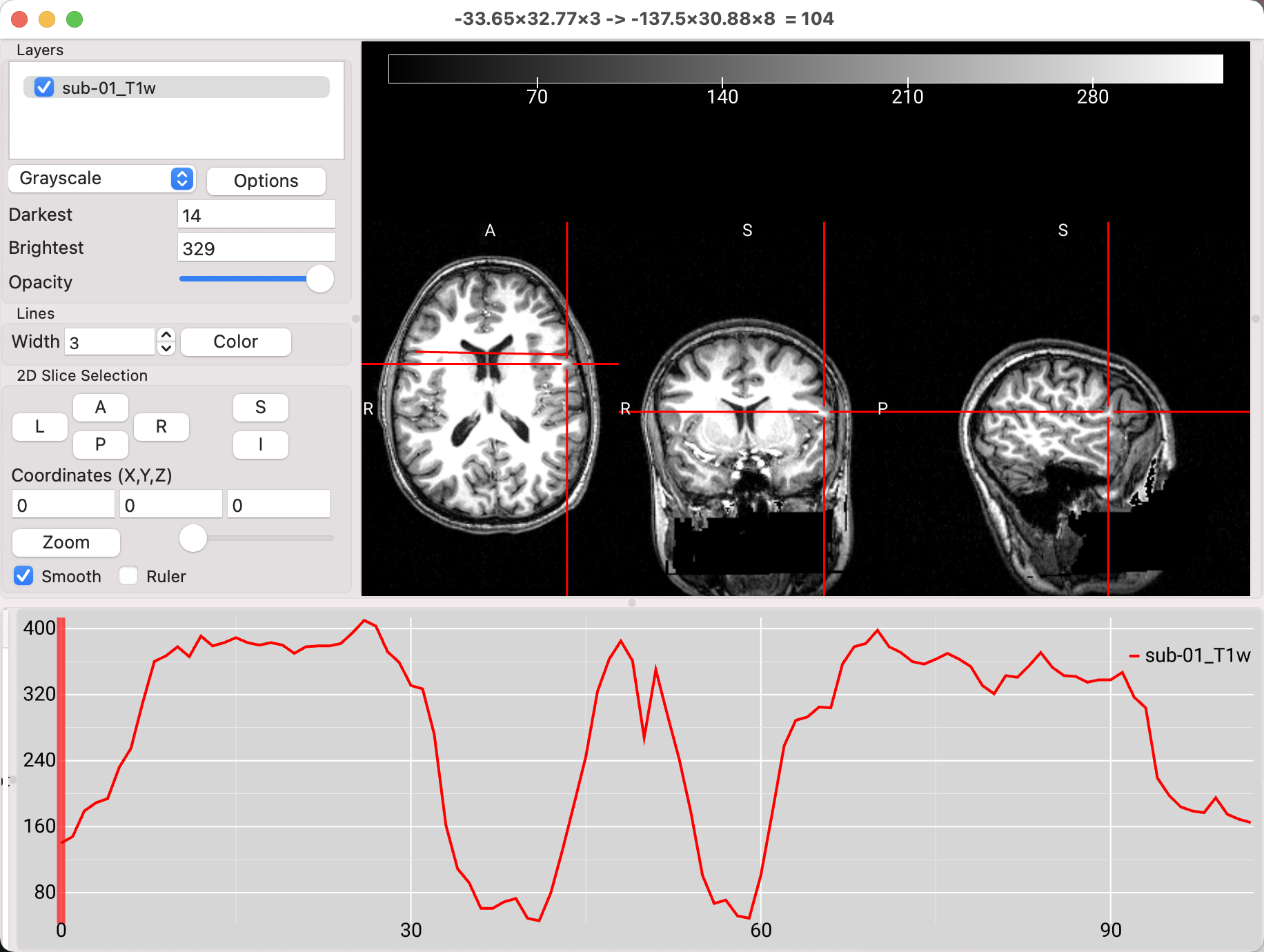
One of the new features in MRIcroGL is the ability to visualize the changes in intensity over multiple slices. First, you will need to find the top of a “hidden” window pane at the bottom of the MRIcroGL viewer; click and drag it up to see another window. Then, find an axial slice that clearly shows both lateral ventricle, click somewhere in the left-hand side of the brain, hold down the option key, and drag the mouse to the right-hand side of the brain. You will see an intensity profile generated in the bottom window, depicting how the intensity changes over the slices that you selected. Note that in this case there are two dips in intensity, indicating where the line you drew crossed over the lower-intensity ventricles.
Loading Multiple Images
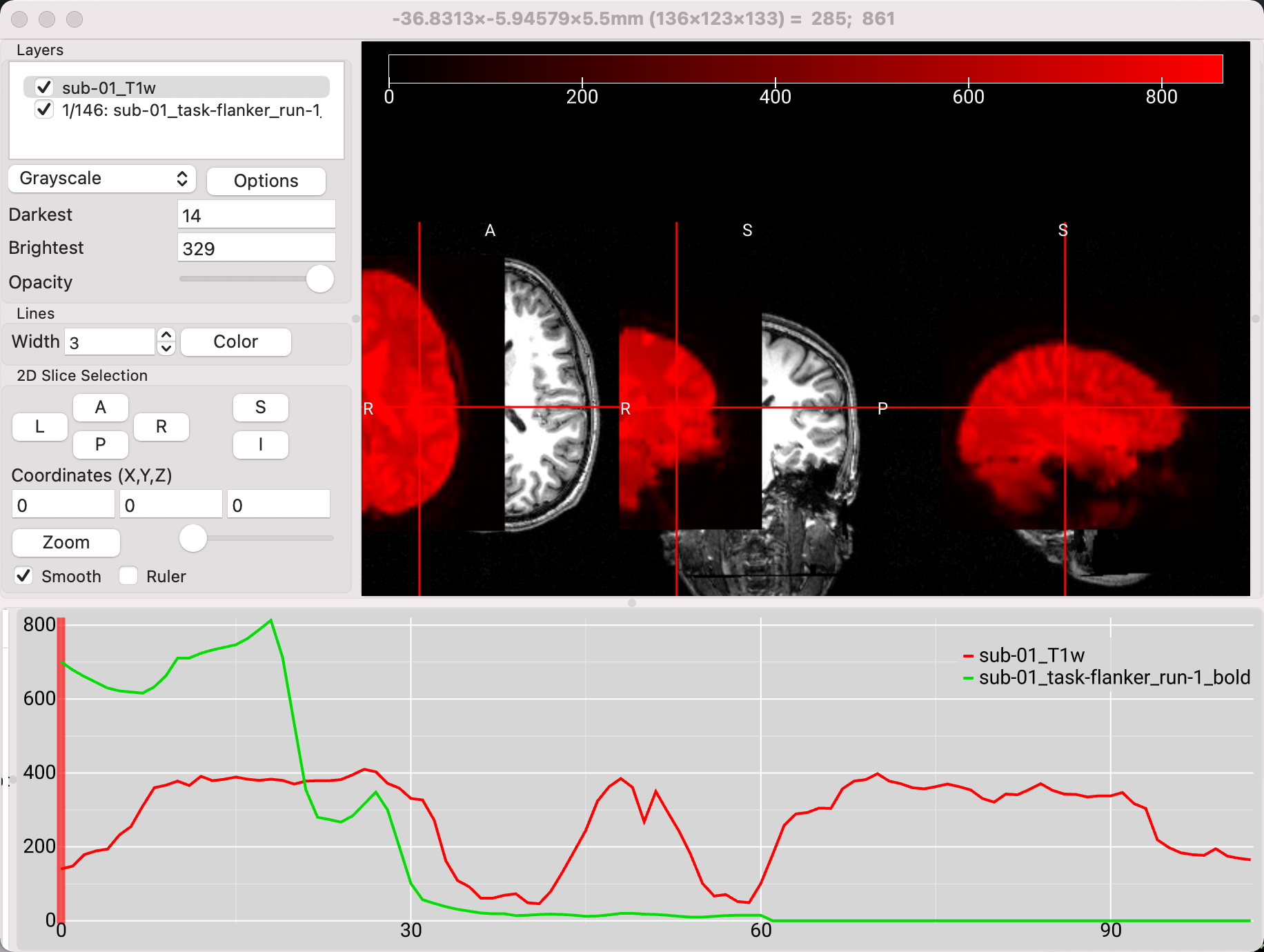
Leaving the anatomical image loaded, click on File -> Add Overlay, and select one of the functional images from the sub-10/func directory. Recall that viewing both the anatomical and functional images can be useful for seeing how far apart the images are, before any preprocessing has been done; images that start farther away from each other may need a larger search area during coregistration in order to find a good fit, or the origins may need to be manually centered before doing any further preprocessing. In this case, the images are quite far away from each other, with the functional image highlighted in red:
After you’ve run coregistration and normalization, you can also use MRIcroGL to evaluate how well the functional and anatomical images are aligned, and how those images in turn are aligned to standardized space. If you’ve run your analyses through FSL, for example, you can find the output from these steps in the reg directory from your feat folder. Open the highres.nii.gz image from subject sub-10’s run1.feat directory, and lower the value of the Brightest field to 800. Then click on File -> Add Overlay, and select the image example_func2highres.nii.gz. You should see something like this:
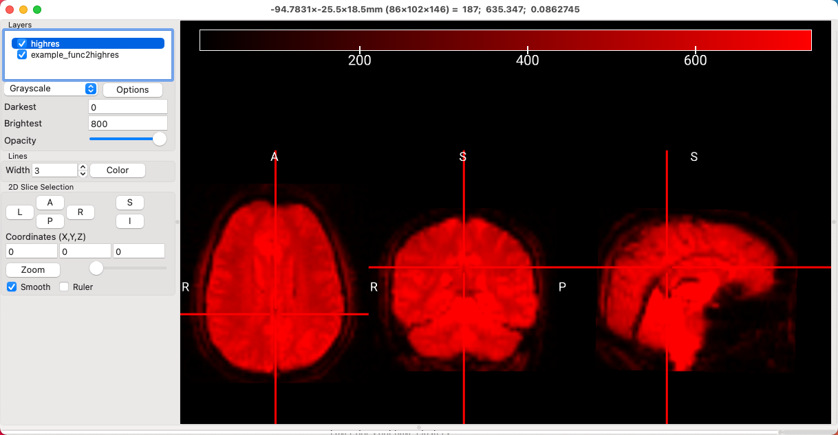
Now there is nearly complete overlap of the functional image on top of the anatomical image, which is what we would expect if the coregistration was successful. However, it is difficult to tell how well some of the internal structures are aligned, such as the ventricles and basal ganglia. (You could toggle the opacity of the overlay, but that would only show whether the outlines of the brains match up.) To see the edges of features such as the sulci, highlight the example_func2highres image, click on Options, and select Find Edges. This will create a new overlay called edge_example_func2highres, and you can see this image more clearly by unchecking the box next to example_func2highres. Now we can see more clearly where the edges of the brains are aligned, and how well the interior structures match up:
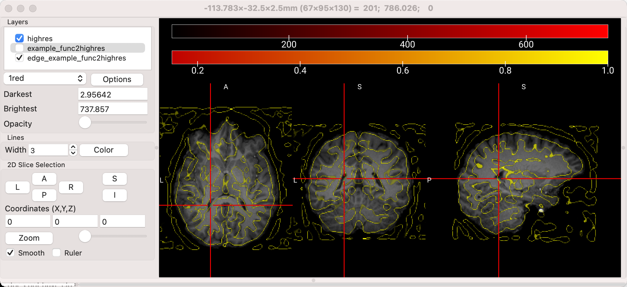
Example of the “Find Edges” feature of MRIcroGL. Note the outline of the ventricles and the basal ganglia in the axial view, and the how the outlines of the sulci are traced.
Video
A video overview of how to view the data can be found here.
Next Steps
Once you have familiarized yourself with how to load anatomical and functional data, you can begin to use the software to overlay statistical maps on a template image; this will be the first step towards creating a publication-quality image of your results. To see how to do that, click the Next button.