MRtrix Tutorial #7: Streamlines
Overview
Having created the interface between the white matter and the grey matter, we are ready to generate streamlines - threads that connect anatomically distinct regions of grey matter. These are estimates of the underlying white matter tracts, and MRtrix uses a probabilistic approach to do this; a large number of streamlines are generated for each voxel of the grey matter / white matter boundary, and then those streamlines are culled based on different criteria that we specify. We will discuss some of the most popular options below.
Anatomically Constrained Tractography
One of MRtrix’s features is Anatomically Constrained Tractography, or ACT. This method will only determine that a streamline is valid if it is biologically plausible. For example, a streamline that terminates in the cerebrospinal fluid will be discarded, since white matter tracts tend to both originate and terminate in grey matter. In other words, the streamlines will be constrained to the white matter. The effect of either including or omitting this step can be seen in the following figure:
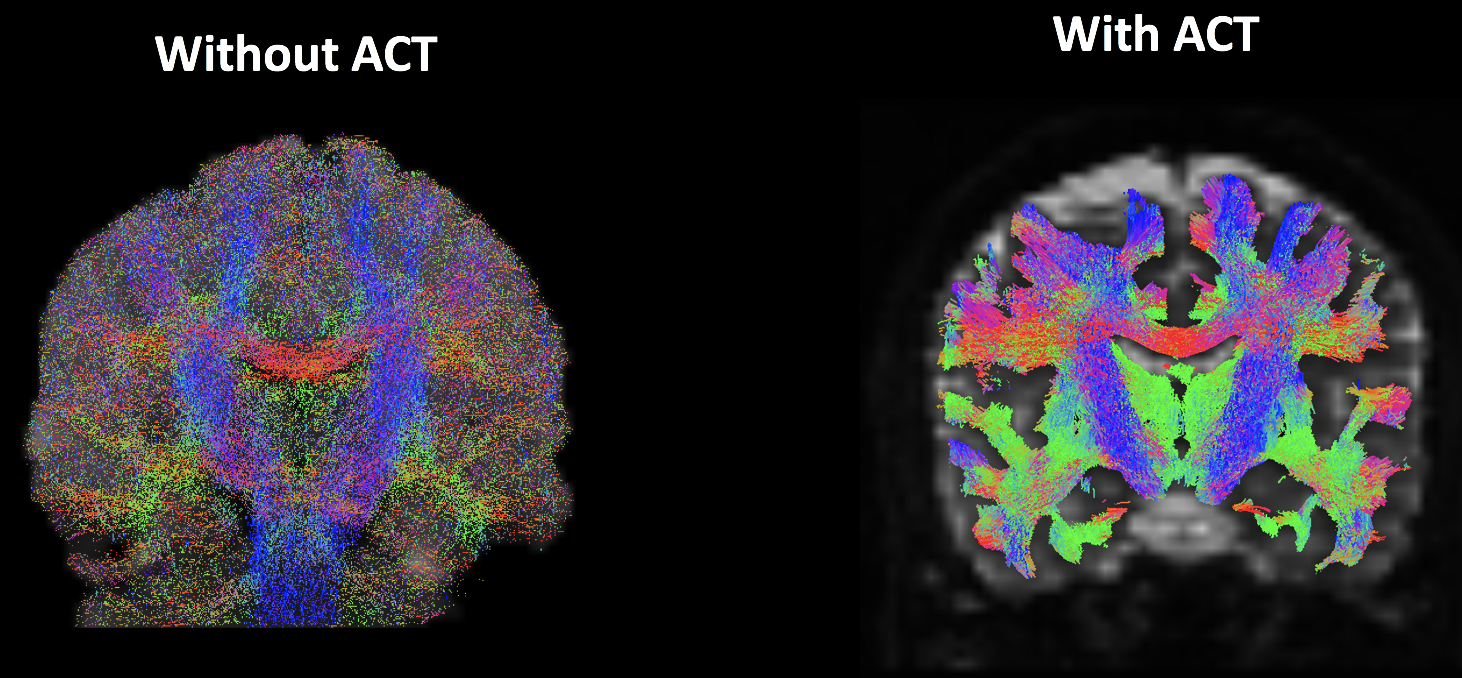
An analysis without (left) and with (right) anatomically constrained tractography. Note how without ACT, the streamlines do tend to congregate within the white matter; however, a large number of them are found within the grey matter and cerebrospinal fluid. Using ACT (right) restricts the streamlines to the white matter tracts that we will want to analyze.
Anatomically constrained tractography isn’t a separate preprocessing step, but rather an option that can be included with the command tckgen, which generates the actual streamlines.
Generating Streamlines with tckgen
MRtrix is able to do both deterministic and probabilistic tractography. In deterministic tractography, the direction of the streamline at each voxel is determined based on the predominant fiber orientation; in other words, the streamline is determined by a single parameter. MRtrix includes multiple options to do this type of deterministic tractography, such as FACT or tensor_det.
The other method, probabilistic tractography, is the default in MRtrix. In this approach, multiple streamlines are generated from seed regions all along the boundary between the grey matter and white matter. The direction of the streamline will most likely follow the predominant fiber orientation density, but not always; due to a large number of samples, some streamlines will follow other directions. This becomes less likely if the FOD is extremely strong in one direction - for example, the FODs within a structure such as the corpus callosum will tend to all be aligned left-to-right - but the sampling becomes more diverse in regions that do not have a predominant fiber orientation.
The default method is to use an algorithm known as iFOD2, which will use a probabilistic streamline approach. Other algorithms can be found at this site, although for the remainder of the tutorial we will use the default of iFOD2.
How Many Streamlines?
There is a trade-off between the number of generated streamlines and the amount of time that it takes. More streamlines result in a more accurate reconstruction of the underlying white-matter tracts, but estimating a large number of them can take a prohibitively long time.
The “correct” number of streamlines to use is still being debated, but at least 10 million or so should be a good starting place:
tckgen -act 5tt_coreg.mif -backtrack -seed_gmwmi gmwmSeed_coreg.mif -nthreads 8 -maxlength 250 -cutoff 0.06 -select 10000000 wmfod_norm.mif tracks_10M.tck
In this command, the “-act” option specifies that we will use the anatomically-segmented image to constrain our analysis to the white matter. “-backtrack” indicates for the current streamline to go back and run the same streamline again if it terminates in a strange place (e.g., the cerebrospinal fluid); “-maxlength” sets the maximum tract length, in voxels, that will be permitted; and “-cutoff” specifies the FOD amplitude for terminating a tract (for example, a value of 0.06 would not permit a streamline to go along an FOD that is lower than that number). “-seed_gmwmi” takes as an input the grey-matter / white-matter boundary that was generated using the 5tt2gmwmi command.
“-nthreads” specifies the number of processing cores you wish to use, in order to speed up the analysis. And finally, “-select” indicates how many total streamlines to generate. Note that a shorthand can be used if you like; instead of, say, 10000000, you can rewrite it as 10000k (meaning “ten thousand thousands”, which equals “ten million”). The last two arguments specify both the input (wmfod_norm.mif) and a label for the output (tracks_10M.tck).
If you want to visualize the output, I recommend extracting a subset of the output by using tckedit:
tckedit tracks_10M.tck -number 200k smallerTracks_200k.tck
This can then be loaded into mrview by using the “-tractography.load” option, which will automatically overlay the smallerTracks_200k.tck file onto the preprocessed diffusion-weighted image:
mrview sub-02_den_preproc_unbiased.mif -tractography.load smallerTracks_200k.tck
This will generate a figure like the following:
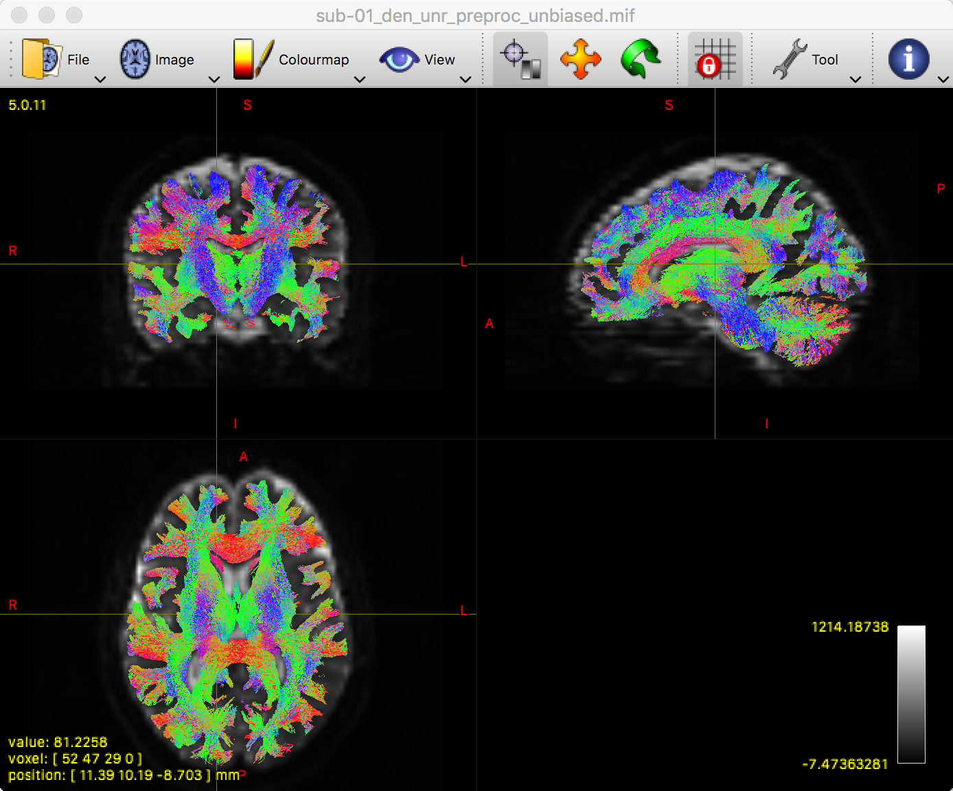
Remember to inspect this image to make sure that the streamlines end where you think they should; in other words, the streamlines should be constrained to the white matter, and they should be color-coded appropriately. For example, the corpus callosum should be mostly red, and the corona radiata should be mostly blue.
Although we have created a diffusion image with reasonable streamlines, also known as a tractogram, we still have a problem with some of the white matter tracts being over-fitted, and others being under-fitted. This can be addressed with the tcksift2 command.
Refining the Streamlines with tcksift2
You may ask why there is any need to modify the streamlines further once we have created our tractogram. The reason is that some tracts will be threaded with more streamlines than others, because the fiber orientation densities are much clearer and more attractive candidates for the probabilistic sampling algorithm that was discussed above. In other words, certain tracts can be over-represented by the amount of streamlines that pass through them not necessarily because they contain more fibers, but because the fibers tend to all be orientated in the same direction.
To counter-balance this overfitting, the command tcksift2 will create a text file containing weights for each voxel in the brain:
tcksift2 -act 5tt_coreg.mif -out_mu sift_mu.txt -out_coeffs sift_coeffs.txt -nthreads 8 tracks_10M.tck wmfod_norm.mif sift_1M.txt
The output from the command, “sift_1M.txt”, can be used with the command tck2connectome to create a matrix of how much each ROI is connected with every other ROI in the brain - a figure known as a connectome - which will weight each ROI. To see how to do that, click the Next button.
Video
For a video overview of streamlines and how to fit them with tckgen, click here.