MRtrix Tutorial #4: Preprocessing
Overview
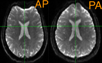
Just like other neuroimaging data, diffusion data should be preprocessed before it is analyzed. Preprocessing removes sources of noise from the image, such as movement artifacts and other distortions. Diffusion data in particular is susceptible to warping artifacts as a result of the phase-encoding direction: In general, the predominant encoding direction - such as Anterior to Posterior, or AP - will make the anterior part of the brain look more “squished”, as though a strong headwind is blowing from the Anterior direction. The opposite is true of the Posterior to Anterior, or PA, phase-encoding direction. Sometimes these distortions are very subtle, but other times they are conspicuous:
The following are common preprocessing steps done with MRtrix. If you have used the software package FSL to analyze diffusion data, note that some of the FSL commands - such as eddy and topup - are used in some of the MRtrix libraries. We will explore that more below.
dwi_denoise
The first preprocessing step we will do is denoise the data by using MRtrix’s dwidenoise command. This requires an input and an output argument, and you also have the option to output the noise map with the -noise option. For example:
dwidenoise sub-02_dwi.mif sub-02_den.mif -noise noise.mif
This command should take a couple of minutes to run.
One quality check is to see whether the residuals load onto any part of the anatomy. If they do, that may indicate that the brain region is disproportionately affected by some kind of artifact or distortion. To calculate this residual, we will use another MRtrix command called mrcalc:
mrcalc sub-02_dwi.mif sub-02_den.mif -subtract residual.mif
You can then inspect the residual map with mrview:
mrview residual.mif
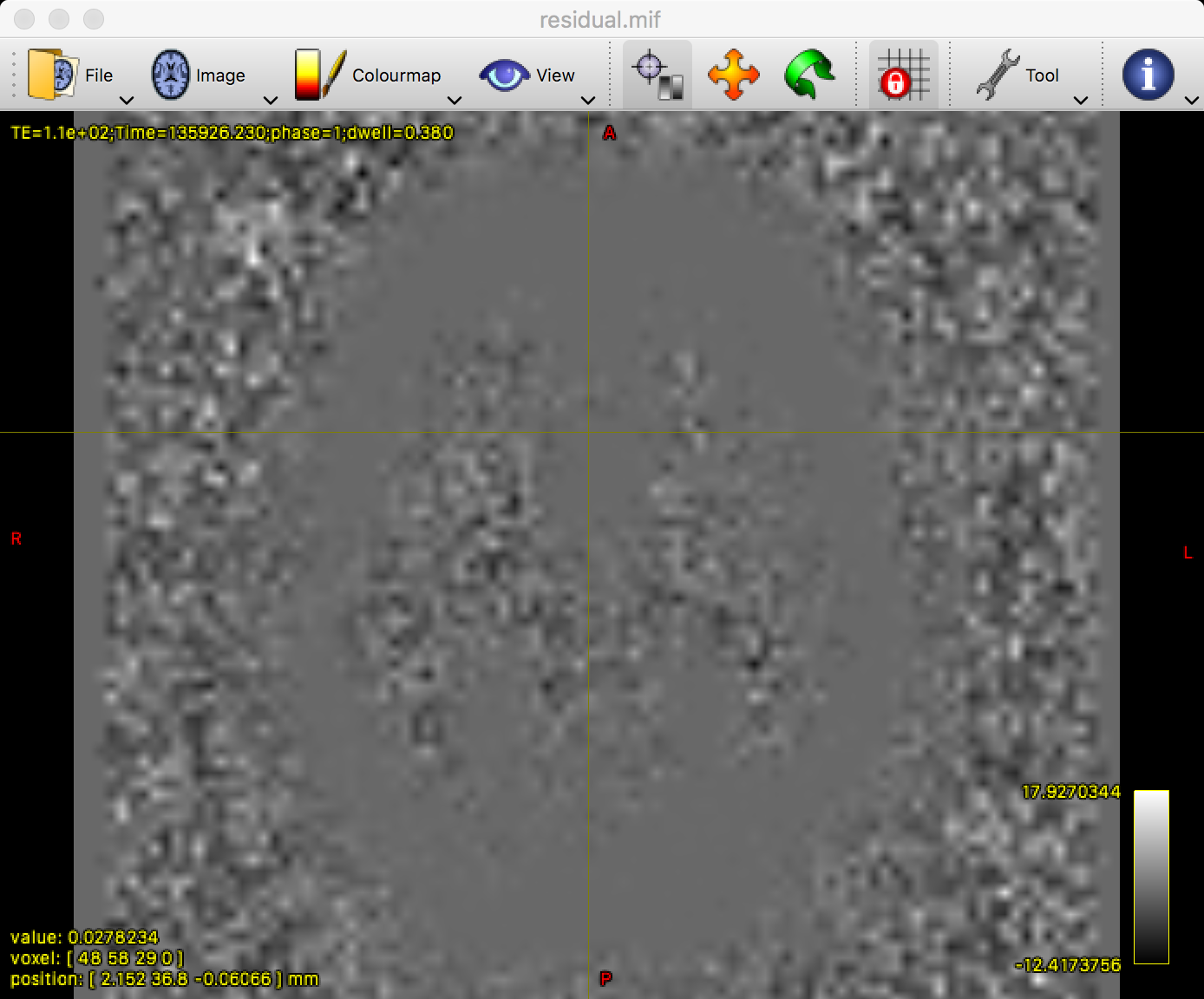
It is common to see a grey outline of the brain, as in the figure above. However, everything within the grey matter and white matter should be relatively uniform and blurry; if you see any clear anatomical landmarks, such as individual gyri or sulci, that may indicate that those parts of the brain have been corrupted by noise. If that happens, you can increase the extent of the denoising filter from the default of 5 to a larger number, such as 7; e.g.,
dwidenoise your_data.mif your_data_denoised_7extent.mif -extent 7 -noise noise.mif
mri_degibbs
An optional preprocessing step is to run mri_degibbs, which removes Gibbs’ ringing artifacts from the data. These artifacts look like ripples in a pond, and are most conspicuous in the images that have a b-value of 0. Look at your diffusion data first with mrview, and determine whether there are any Gibbs artifacts; if there are, then you can run mrdegibbs by specifying both an input file and output file, e.g.:
mrdegibbs sub-02_den.mif sub-02_den_unr.mif
As always, inspect the data both before and after with mrview to determine whether the preprocessing step made the data better, worse, or had no effect.
If you don’t see any Gibbs artifacts in your data, then I would recommend omitting this step; we won’t be using it for the rest of the tutorial.
Extracting the Reverse Phase-Encoded Images
Most diffusion datasets are composed of two separate imaging files: One that is acquired with a primary phase-encoding direction, and one that is acquired with a reverse phase-encoding direction. The primary phase-encoding direction is used to acquire the majority of the diffusion images at different b-values. The reverse-phase encoded file, on the other hand, is used to unwarp any of the distortions that are present in the primary phase-encoded file.
To understand how this works, imagine that you are using a blow dryer on your hair. Let’s say that you have the blow dryer pointed at the back of your head, and it blows your hair forward, onto the front of your face; let’s call this the posterior-to-anterior (PA) phase-encoding direction. Right now your hair looks like a mess, and you want to undo the effects of the air blowing from the back of your head to the front of your head. So you point the blow dryer at the front of your face, and it blows your hair back. If you take the average between the two of those blow dryings, your hair should be back in its normal position.
Similarly, we use both phase-encoding directions to create a sort of average between the two. We know that both types of phase-encoding will introduce two separate and opposite distortions into the data, but we can use unwarping to cancel them out.
Our first step is to convert the reverse phase-encoded NIFTI file into .mif format. We will also add its b-values and b-vectors into the header:
mrconvert sub-CON02_ses-preop_acq-PA_dwi.nii.gz PA.mif
mrconvert PA.mif -fslgrad sub-02_PA.bvec sub-02_PA.bval - | mrmath - mean mean_b0_PA.mif -axis 3
Next, we extract the b-values from the primary phase-encoded image, and then combine the two with mrcat:
dwiextract sub-02_den.mif - -bzero | mrmath - mean mean_b0_AP.mif -axis 3
mrcat mean_b0_AP.mif mean_b0_PA.mif -axis 3 b0_pair.mif
This will create a new image, “b0_pair.mif”, which contains both of the average b=0 images for both phase-encoded images.
Putting It All Together: Preprocessing with dwipreproc
We now have everything we need to run the main preprocessing step, which is called by dwipreproc. For the most part, this command is a wrapper that uses FSL commands such as topup and eddy to unwarp the data and remove eddy currents. For this tutorial, we will use the following line of code:
dwifslpreproc sub-02_den.mif sub-02_den_preproc.mif -nocleanup -pe_dir AP -rpe_pair -se_epi b0_pair.mif -eddy_options " --slm=linear --data_is_shelled"
The first arguments are the input and output; the second option, -nocleanup, will keep the temporary processing folder which contains a few files we will examine later. -pe_dir AP signalizes that the primary phase-encoding direction is anterior-to-posterior, and -rpe_pair combined with the -se_epi options indicates that the following input file (i.e., “b0_pair.mif”) is a pair of spin-echo images that were acquired with reverse phase-encoding directions. Lastly, -eddy_options specifies options that are specific to the FSL command eddy. You can visit the eddy user guide for more options and details about what they do. For now, we will only use the options --slm=linear (which can be useful for data that was acquired with less than 60 directions) and --data_is_shelled (which indicates that the diffusion data was acquired with multiple b-values).
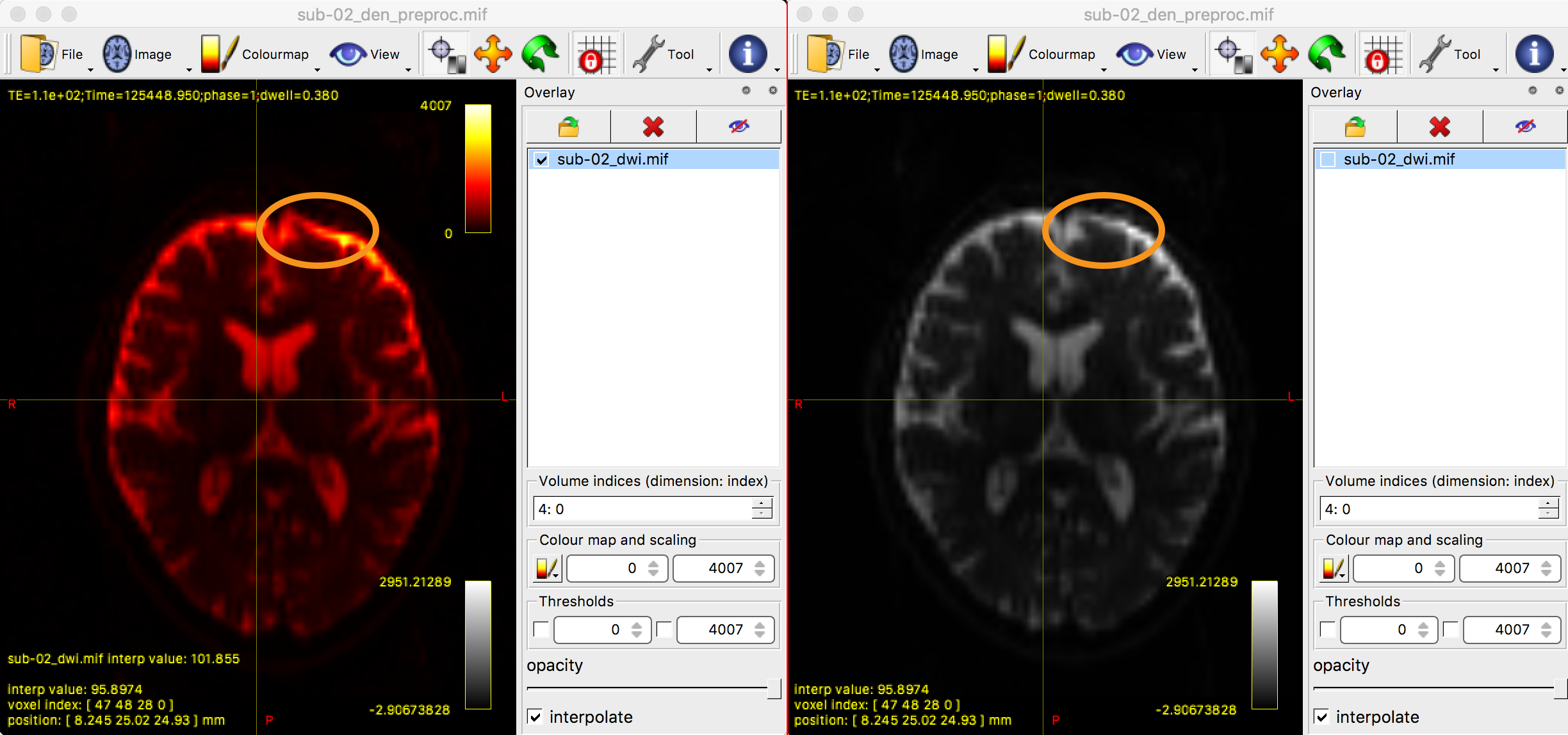
This command can take several hours to run, depending on the speed of your computer. For an iMac with 8 processing cores, it takes roughly 2 hours. When it has finished, examine the output to see how eddy current correction and unwarping have changed the data; ideally, you should see more signal restored in regions such as the orbitofrontal cortex, which is particularly susceptible to signal dropout:
mrview sub-02_den_preproc.mif -overlay.load sub-02_dwi.mif
This command will display the newly preprocessed data, with the original diffusion data overlaid on top of it and colored in red. To see how the eddy currents were unwarped, open the Overlays tab and click on the box next to the image sub-02_dwi.mif. You should see a noticeable difference between the two images, especially in the frontal lobes of the brain near the eyes, which are most susceptible to eddy currents.
Checking for Corrupt Slices
One of the options in the dwifslpreproc command, “-nocleanup”, retained a directory with the string “tmp” in its title. Within this folder is a file called dwi_post_eddy.eddy_outlier_map, which contains strings of 0’s and 1’s. Each 1 represents a slice that is an outlier, either because of too much motion, eddy currents, or something else.
The following code, run from the dwi directory, will navigate into the “tmp” folder and calculate the percentage of outlier slices:
cd dwifslpreproc-tmp-*
totalSlices=`mrinfo dwi.mif | grep Dimensions | awk '{print $6 * $8}'`
totalOutliers=`awk '{ for(i=1;i<=NF;i++)sum+=$i } END { print sum }' dwi_post_eddy.eddy_outlier_map`
echo "If the following number is greater than 10, you may have to discard this subject because of too much motion or corrupted slices"
echo "scale=5; ($totalOutliers / $totalSlices * 100)/1" | bc | tee percentageOutliers.txt
cd ..
The first two lines navigate into the “tmp” directory and calculate the total number of slices by multiplying the number of slices for a single volume by the total number of volumes in the dataset. The total number of 1’s in the outlier map is then calculated, and the percentage of outlier slices is generated by dividing the number of outlier slices by the total number of slices. If this number is greater than 10 - i.e., if more than 10 percent of the slices are flagged as outliers - you should consider removing the subject from further analyses.
Generating a Mask
As with fMRI analysis, it is useful to create a mask to restrict your analysis only to brain voxels; this will speed up the rest of your analyses.
To do that, it can be useful to run a command beforehand called dwibiascorrect. This can remove inhomogeneities detected in the data that can lead to a better mask estimation. However, it can in some cases lead to a worse estimation; as with all of the preprocessing steps, you should check it before and after each step:
dwibiascorrect ants sub-02_den_preproc.mif sub-02_den_preproc_unbiased.mif -bias bias.mif
Note
The command above uses the -ants option, which requires that ANTs be installed on your system. I recommend this program, but in case you are unable to install it, you can replace it with the -fsl option.
You are now ready to create the mask with dwi2mask, which will restrict your analysis to voxels that are located within the brain:
dwi2mask sub-02_den_preproc_unbiased.mif mask.mif
Check the output of this command by typing:
mrview mask.mif
You should see something like the following:
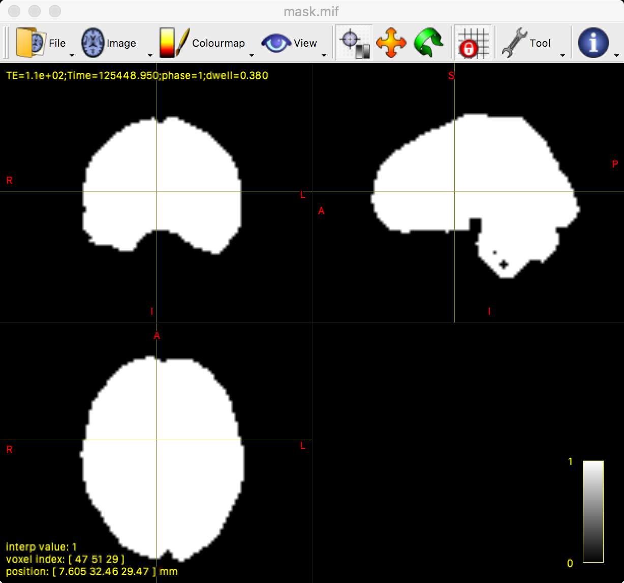
MRtrix’s dwi2mask command works well in most scenarios. However, you can see from the above image that there are a few holes in the mask within the brainstem and the cerebellum. You may be uninterested in these regions, but it is still a good idea to make sure the mask doesn’t have any holes anywhere.
To that end, you could use a command such as FSL’s bet2. For example, you could use the following code to convert the unbiased diffusion-weighted image to NIFTI format, create a mask with bet2, and then convert the mask to .mif format:
mrconvert sub-02_den_preproc_unbiased.mif sub-02_unbiased.nii
bet2 sub-02_unbiased.nii sub-02_masked -m -f 0.7
mrconvert sub-02_masked_mask.nii.gz mask.mif
You may have to experiment with the fractional intensity threshold (specified by -f) in order to generate a mask that you are satisfied with. In my experience, this can vary between 0.2 and 0.7 for most brains in order to generate an adequate mask.
Video
A video overview of preprocessing in MRtrix can be found here.
Next Steps
Now that we have our preprocessed diffusion data and a mask, we are ready to do constrained spherical deconvolution, which we cover in the next chapter.