Meta-Analysis Tutorial #1: Activation Likelihood Estimation with GingerALE
Overview
The earliest meta-analysis tool developed for neuroimaging data was a method called Activation Likelihood Estimation, or ALE. First demonstrated by Turkeltaub et al. in 2002, ALE estimates the likelihood of overlap between the activation of different studies (also referred to as the “concordance” between the studies) as compared to a null distribution computed over several permutations. In this way, it is similar to how significant clusters are calculated for fMRI studies: The cluster reported in your study is compared to a distribution of clusters generated at random, and the cluster is deemed significant if it is larger than the largest 5% of randomly generated clusters.
Further modifications to Turkeltaub’s original ALE study led to a new meta-analysis package called GingerALE. This is part of a suite of packages called BrainMap, which also includes the auxiliary programs Scribe and Sleuth; for now, however, we will just focus on GingerALE, demonstrating how to replicate the results of another meta-analysis, and then to contrast two meta-analyses to determine where there is either overlap or differences between them. And to do that, we first need to briefly review the GingerALE Interface.
The GingerALE Interface
The GingerALE package can be downloaded by clicking on this link and choosing the version matching your operating system; downloading and installing the package is straightforward, and should only take a couple of minutes. Click on the file once you have downloaded it, and then click and drag the GingerALE icon into your Applications directory, which allows you to open the package by using your Finder to search for “GingerALE”. Click on the software package result that appears, which will open the GingerALE interface.
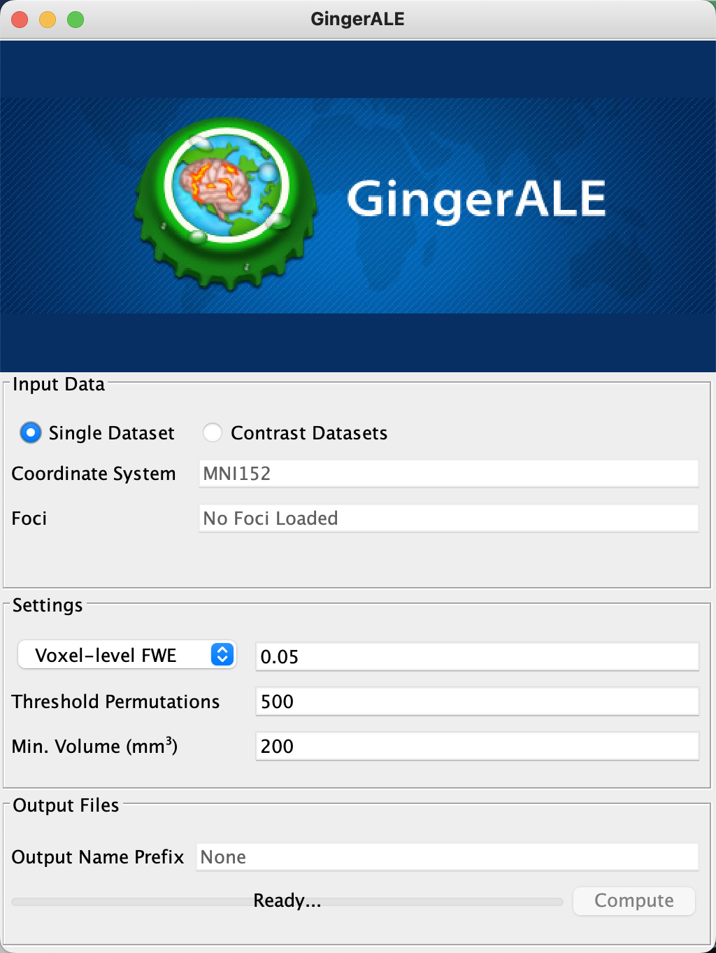
The radio button by default is set to “Single Dataset”, which is what we will start with; that is, we will test whether the results of several different studies examining the same contrast have significant overlap. Not all of the studies need to use the exact same contrast, it should be noted; there will be differences in experimental design, as well as number of subjects and number of trials. But each study that is included in the meta-analysis ought to tap into the same underlying cognitive phenomenon, whether it be working memory, cognitive control, and so forth. In the Turkeltaub et al. 2002 paper discussed above, for example, they included studies which measured where reading aloud elicited higher PET signals in the brain, relative to some control condition. Here is a partial list of those controls:
Silent Reading
Fixation
Rest
As you can see, there were a variety of control conditions, which entails more variability when comparing studies; but since all of the contrasts used Reading, we can combine them into a meta-analysis. It is up to you to define the criteria for which studies you will include in your meta-analysis.
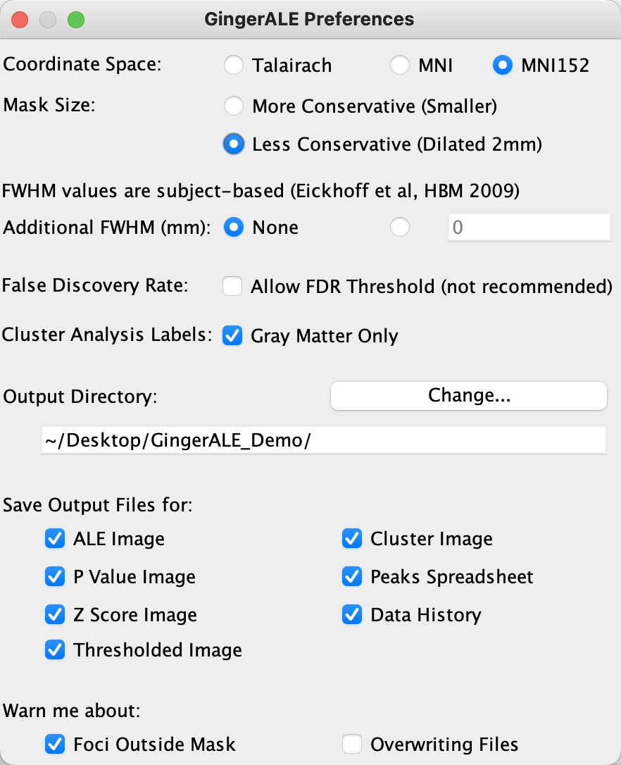
You may notice that the default coordinate system listed by GingerALE is “Talairach”, a template used by many neuroimaging studies in the 1990s and early 2000s, but which has been superseded by a newer template space, Montreal Neurological Institute (or MNI). To change the coordinate space to MNI, click on GingerALE -> Settings, and select the radio button next to “MNI152” - a variation of the MNI template composed of an average of 152 subjects, and with slightly different dimensions than MNI.
The next field, “Mask Size”, specifies whether to make the mask bigger or smaller - that is, to make the space of our analysis included more or fewer voxels. It may be the case, for example, that one of the studies included in your meta-analysis used a slightly bigger mask than usual, and that this in turn led to a peak activation being located beyond the edge of a more conservative mask used by the other studies. Later on you may find that the foci you want to use in your study fall outside the default, more conservative mask used by GingerALE, and you can change that here.
All of the other options are mostly self-explanatory, and the defaults should be left as they are. The only other option you may want to change is the “Output Directory” field, which by default points to the home directory. To better organize our results, create a new directory on your Desktop called GingerALE_Demo, and then select this folder as your output directory. When you are finished, your GingerALE preferences should look like this:
Once you have closed the Preferences window, you may see your changes reflected in the main GingerALE interface; for example, the coordinate system will change from Talairach to MNI152. Passing over the Foci field for now, you will see the Settings field, with a drop-down menu showing options for different correction methods. The first one in the list, P Value, is an uncorrected value applied to all of the voxels, and unless you are exploring your meta-analysis data without the intent to publish, I would not recommend using it.
The second option, Voxel-level FWE, is similar to Bonferroni correction for fMRI data; it ensures that no more than a specified fraction of ALE scores exceed a given value. Once you choose this option, you will see additional fields; the one next to Voxel-level FWE is your alpha level at each voxel, while Threshold Permutations specifies how many null datasets will be simulated to build up the null distribution. The last field, Min. Volume (mm3) will remove any remaining voxels that do not belong to a cluster as large or larger than the volume entered.
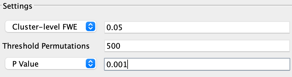
Similar to cluster-based thresholding for fMRI data, the last option, Cluster-level FWE, allows you to specify the cluster-forming threshold in the field next to P Value (which should be kept at 0.001), and the alpha level in the field next to Cluster-level FWE for the resulting clusters (which I recommend setting to the nominal 0.05 value). As with the previous option of Voxel-level FWE, the number of threshold permutations determines the amount of null clusters that are created in order to create a null distribution. For the purposes of this tutorial, let’s stick with Cluster-level FWE as our correction method.
Note
If you are testing GingerALE for the first time, you may decide to use fewer permutations, e.g., 100 or 200, to quickly create a meta-analysis map. For most published analyses, permutations of 1000 or more are commonly used (e.g., Papitto et al., 2020; Hardwick et al., 2018; Teghil et al., 2019).
Creating Foci Files
Once you have gathered a list of studies you want to include in your meta-analysis, you will also need to extract the foci, or peaks, for the contrasts that they reported in their paper. There are tools on the Brainmap website designed to automate this task for you, although you can extract the peaks manually if you wish. In any case, the foci need to be formatted in a particular way in order to be used with GingerALE, and a representative example can be found in the GingerALE manual:
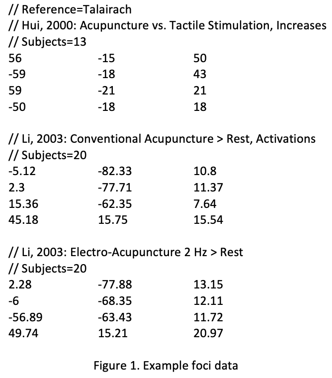
From this sample file, we can see that it requires the following fields:
Reference space, in which all of the coordinates have been reported. Note that if different studies report their coordinates in different spaces, you can convert them to the same space by clicking
Tools -> Convert Foci, selecting the file you would like to convert, and choosing the appropriate conversion - for example, Talairach to MNI.Listing the study name, followed by the contrast reported in that study whose coordinate you are reporting.
Number of subjects in the study
List of coordinates in x-y-z format for each foci reported in the study.
Note that the reference space field is listed only once at the beginning of the file, and that this field, along with the fields listing the study name and the number of subjects, are preceded by two forward slashes (”//”). Each set of coordinates is listed on a separate line, while a carriage return separates each study.
Let’s use this example file to run a small GingerALE meta-analysis. Either transcribe or copy and paste the values into a text file, using a program such as Macintosh’s TextEdit. (Be sure to remove the Rich Text Formatting by selecting Format -> Make Plain Text, or else GingerALE won’t be able to read the file.) Save the file into your GingerALE_Demo folder as Acupuncture_Foci.txt.
Note
If you do copy and paste the values from the GingerALE manual, or from one paper’s table into your text file, make sure that the negative signs are formatted correctly; e.g., copying the negative signs from another paper may be represented as dashes when they are pasted into the text file. If you run into an error with GingerALE unable to interpret these signs, using TextEdit, select Edit -> Find -> Find and Replace. Copy one of the dashes in the Find field, and enter a hyphen (i.e., negative sign) into the Replace field, and click the All button.
Running the Analysis
Now that you have the materials you need for the meta-analysis, open GingerALE and click File -> Open Foci. Select the Acupuncture_Foci.txt file you created, and click Open. When you see a window asking you to change the coordinate system, select Change to Talairach; you may have noticed that the coordinate system specified in the foci file was Talairach, and you should use the corresponding template space for the analysis.
You will notice that the field next to Foci now displays the file you loaded, and it has detected 12 foci across 3 experiments, which you can verify by reading the foci file; the field next to Output Name Prefix has also been changed to the same name as the foci file, although you can modify it if you wish. Click the Compute button, and wait a few minutes for GingerALE to calculate the meta-analysis maps; the output of the analysis is annotated below, which is copied from the GingerALE user manual:
ALE Image: contains the unthresholded ALE values, one computed at every voxel in the brain. The file name used to save this file will be your “Output Name Prefix” setting and the suffix “_ALE.nii”
P Value Image: contains each voxel’s unthresholded P value. File name suffix: “_P.nii”
Thresholded Image: ALE map threshold at a given alpha value. This is considered the final output image, and is used as the input for contrast analyses. It has a variable file name, depending on the thresholding method and value chosen. For example, when using FDR pN < 0.01, the suffix would be “_ALE_pN01.nii”. It could also be “_ALE_p001.nii” or “_ALE_FWE05.nii”, etc.
Cluster Image: The first step in cluster analysis is identifying the contiguous non‐zero regions in the thresholded image. Each voxel in each region is given an integer value, according to which cluster it is in. The clusters are sorted by size, with #1 assigned to the largest cluster. Suffix: “_clust.nii”
Cluster Spreadsheet: An excel document with 10 columns of information about the result’s clusters:
cluster number, with the largest at #1
(2) volume of cluster in mm3 (3‐5) x,y,z values of the weighted center of mass (6) maximum ALE value observed in the cluster (7‐9) x,y,z values of the location of the maximum ALE value (10) Talairach Daemon anatomical label associated with the peak coordinates If your preferences are for a cluster analysis to contain all extrema, then columns 6‐10 will be repeated in a new row with information on each local maximum. Output suffix: “_clust.xls” * Data History: A text file that contains all the parameters and output file names used in the analysis. It also includes additional information about the different stages of analysis, such as the FWHM value range and the total non‐zero volume in the thresholded image. It also includes an expanded cluster analysis, with all of the information from the spreadsheet as well as cluster extent and a volumetric Talairach Label analysis. File name suffix: “_clust.txt”
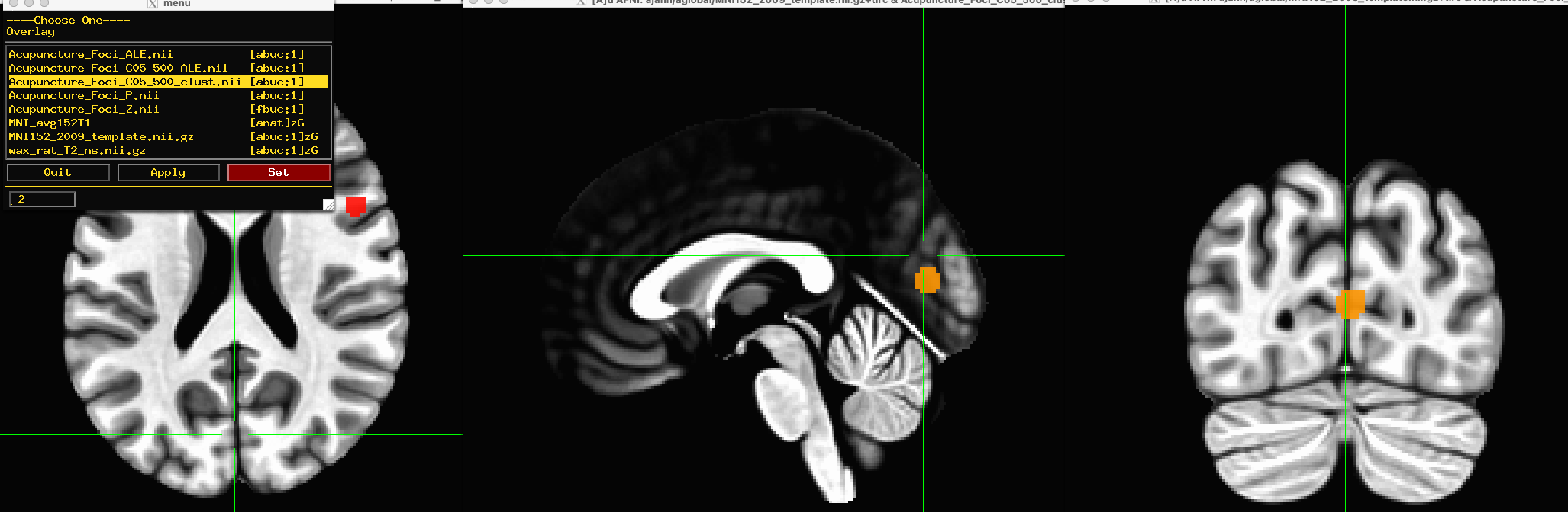
When the analysis has finished, you can navigate into the directory and examine the output with any viewing software that you like; in this case, I will use AFNI. Using the MNI152_2009_template as an Underlay image, you can view any of the output images as an Overlay. The most useful one for our purposes of meta-analysis would be the file Acupuncture_Foci_C05_500_clust.nii, which is the cluster-corrected image that shows where there is significant overlap between the foci of the different studies. In this case we can see two distinct clusters, one in the occipital lobe and one in the inferior frontal gyrus. For exact coordinates of the peaks of each of these clusters, you can open the spreadsheet Acupuncture_Foci_C05_500_peaks.xls, which was also created in the output directory as a result of the analysis.
Replicating the Meta-Analysis of Kumar et al., 2016
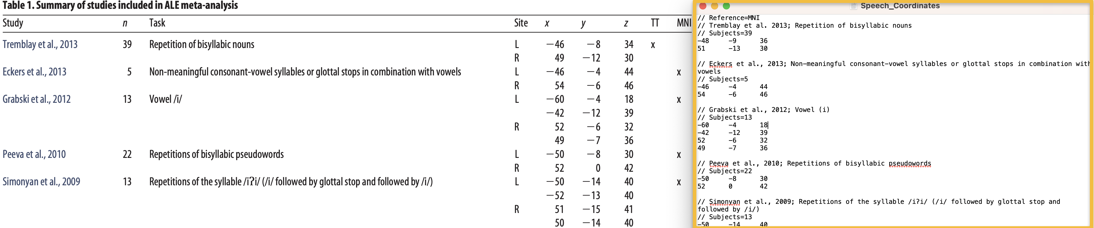
Having used GingerALE to perform a small meta-analysis, let’s expand our scope by using the coordinates reported in a paper by Kumar et al., 2016 which were drawn from several studies examining speech production. The tasks used in these studies, which are listed in Table 1 of the paper, range from saying nouns, vowels, pseudowords, and different kinds of vowel and consonant sequences.
In fact, it is this table that we will draw all of our coordinates from, in order to replicate their meta-analysis. This may take some time to transcribe it by hand into a text file, but it is useful to do this a couple of times to get used to the feel of creating your own set of coordinates, which may not always be available in databases such as Sleuth which extract the coordinates automatically.
As you create the foci file, it should look something like this, with the original paper and the text file displayed side by side:
Note
The Kumar et al. paper lists the space in which each set of coordinates are reported, some of which are in Talairach-Tournoux (TT) space. These coordinates can be converted to MNI using any one of the converters found online, such as this one. Once you are done converting all of the required coordinates, create a new folder called Kumar_Replication, and within that folder save the coordinates file as Speech_Coordinates.txt. Also make sure to change the GingerALE settings to write the output into the Kumar_Replication folder.
From the Methods section of the paper, we learn that the authors performed their meta-analysis with GingerALE as well, using “a familywise error-corrected p = 0.01 with minimum cluster size [sic.] of 200mm^3”. To replicate this we should therefore use the Voxel-level FWE correction method, setting the alpha level to 0.01. (The Min. Volume field should be set to 200 as the default, and so does not need to be changed in this case.) Then, load the foci file and click Compute. This analysis should only take a few minutes.
When the analysis is complete, overlay the cluster-corrected results (i.e., Speech_Coordinates_FWE05_500_ALE.nii) on a template MNI brain; you should see significant ALE overlap in the bilateral laryngeal motor cortex (around area 4 of the motor cortex), similar to what they display in Figure 1 of the paper.
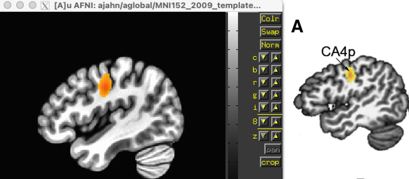
Comparison of the results from the current meta-analysis (left) with the results reported in the Kumar et al. 2016 paper (right).
Using Sleuth to Create Study Coordinates for Music and Sounds
While an activation likelihood map for a single contrast can be useful in itself, you may also want to compare these maps against another cognitive process. To demonstrate this, we will use another software package available on Brainmaps.org, called Sleuth. Click on this link, and download the version of Sleuth that is compatible with your operating system. Then, click here to create an account, which should only take a minute or so. Once this is done, open Sleuth and log in with your new username and password; this will grant you access to the Brainmap database.
Within the panel labeled “Choose your search criteria”, you are able to add as many criteria as you like. The number of options may seem overwhelming, but if you have a good idea of the limits you would like to set on which foci are generated in the search - for example, only studies that have at least twenty subjects, or which fall within one of the hemispheres - you can set them here. The focus of your search, however, probably will use the Conditions option as the first filter, followed by either Stimulus Type or Stimulus Content. You can then look at the resulting options in the dropdown menu at the right, and choose whichever one best suits your analysis. In this case, I will choose Conditions -> Stimulus Type -> is -> Sounds (Environmental), and click the Search button. After a few moments of retrieving the citations, you can proceed to the next tab in the Sleuth window, called Results. Here is a listing of all the studies that were extracted using the filters you specified, providing the article’s year, journal, and list of authors. You can highlight any of the studies and click on the options Citation, Prose Description, and Experiment Info to read more details about the study. In this case, we will assume that we want to include all of the studies, and click on Download All.
Once the papers are downloaded, Sleuth will move to the Workspace tab, in which you can see the number of foci reported in each paper and a color code for each study. By default, all of the boxes next to each paper are checked; if you then click on View Plot, you will see all of the foci plotted on three orthogonal slices in the brain, color-coded by which study they belong to.
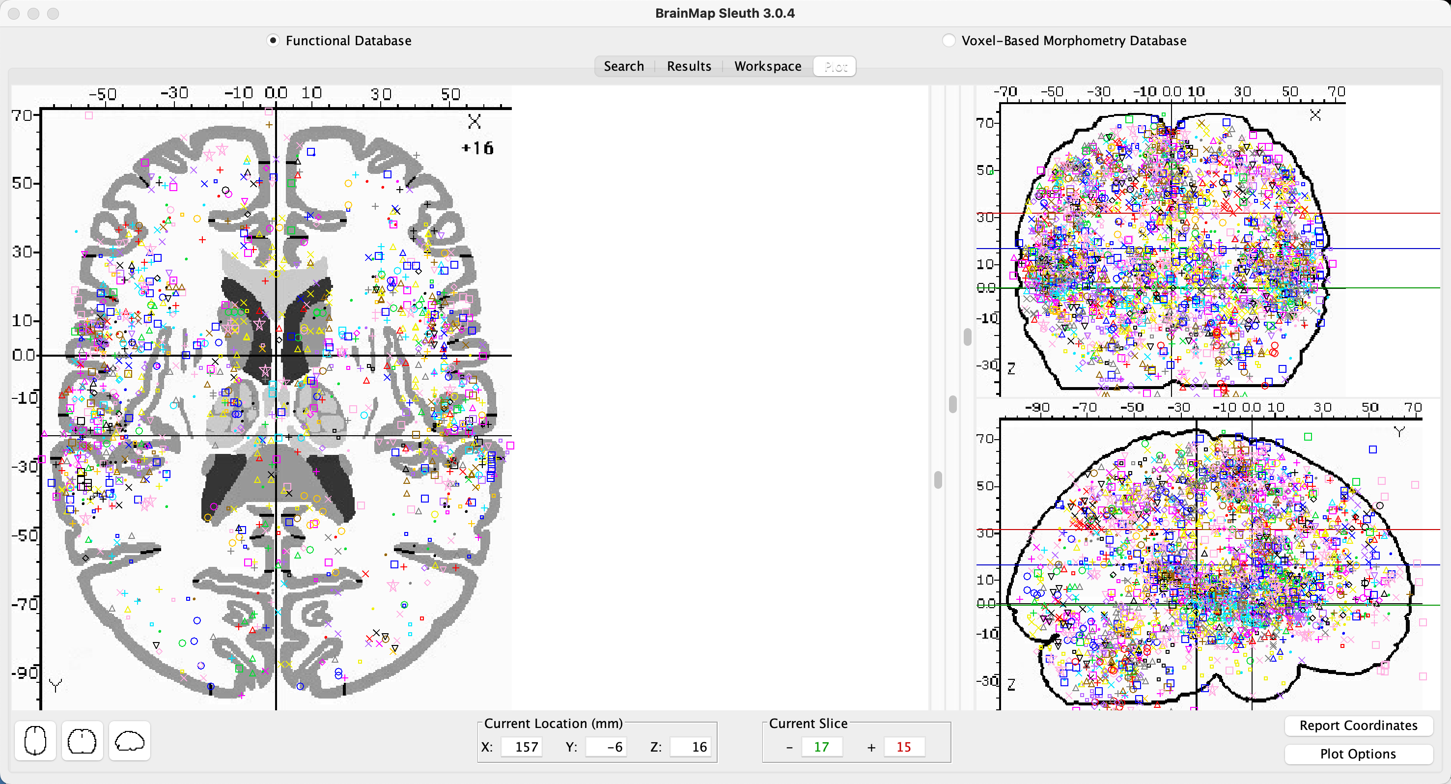
Example foci plot for “Sounds” experiments. The left panel contains a close-up of one of the three orthogonal views, which can be changed by clicking on any of the other views in the bottom-left corner. The other two orthogonal views are displayed in the panel to the right. There are three sliders in the middle of the Plot pane: The sliders on the left and right set the limits for the bottom and top boundaries of the slice, while the middle slider allows you to move the entire slice through the orthogonal view in the left pane.
After you have reviewed the foci and determined whether they are suitable to use, you can export the foci into a text file by clicking on Export -> Locations (GingerALE Text) from the top of your screen. You may also find it helpful to first click on Export -> Export to MNI to ensure that the coordinates are first converted to MNI space. Create a new folder called Sounds_Music_Comparison, and save the file as Sounds_Coordinates.txt in that folder. In order to compare this to a related condition - for example, Music - we can re-run the Sleuth program by clicking on the Search tab and changing the search criteria to Conditions -> Stimulus Type -> is -> Music. After that, perform the same steps as you did above to generate the Sound_Coordinates.txt file, but in this case save the coordinates as Music_Coordinates.txt.
Note
When creating a new foci file for the Music condition, you may need to close Sleuth and re-open it; this flushes the previous coordinates out of memory, so that the new coordinates will not be concatenated to the ones from the previous analysis.
Performing a Meta-Analysis of Music and Sound Coordinates
The analysis of these datasets are identical to the first; once you have opened the Foci file for the Sounds_Coordinates.txt file, click Compute. (To keep the analyses as similar as possible, leave the correction parameters the same; viz., Voxel-level FWE of 0.05, 500 Permutations, and 200mm3 volume. Also make sure to reset the Output Directory through the GingerALE Preferences panel.) As with the previous analysis, load the cluster-corrected maps in a software viewer of your choice to make sure that the activations are where you expect them to be - such as the primary auditory cortex of the auditory lobes. Then, do the same analysis with the Music_Coordinates.txt file.
Our next task is to create a pooled coordinates file, which is just a concatenation of the Speech and Sounds coordinate files we have already written. You are welcome to do this by hand, or, if you would like to have GingerALE do it for you, click on the Contrast Datasets radio button, load both of the thresholded ALE maps (in our case, click on File -> Open ALE Image 1 and load the file Music_Coordinates_FWE05_500_ALE.nii, and then click File -> Open ALE Image 2 and load Sounds_Coordinates_FWE05_500_ALE.nii), and then click on File -> Merge & Save Foci. Save the file as pooled.txt in the Sounds_Music_Comparison directory.
The analysis of this pooled file is the same as analyzing the previous sets of foci: Click on the radio button next to Single Dataset, and then select File -> Open Foci and open the pooled.txt file. Use the same settings as before, and click the Compute button. The analysis may take up to a half hour to complete.
When it has finished, click on Contrast Datasets again. Click on File -> Open ALE Image 1, and select Music_Coordinates_FWE05_500_ALE; then, click on File -> Open ALE Image 2 and select Sounds_Coordinates_FWE05_500_ALE. The last file we need to load is the pooled_FWE05_500_ALE, which you can select by clicking File -> Open Pooled ALE Image. Click Compute.
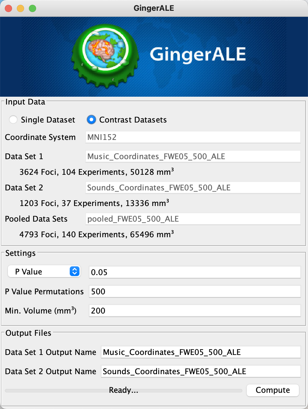
Loading the images for a Contrast meta-analysis.
The Sounds_Music_Comparison directory should look like this when you have finished the analysis:
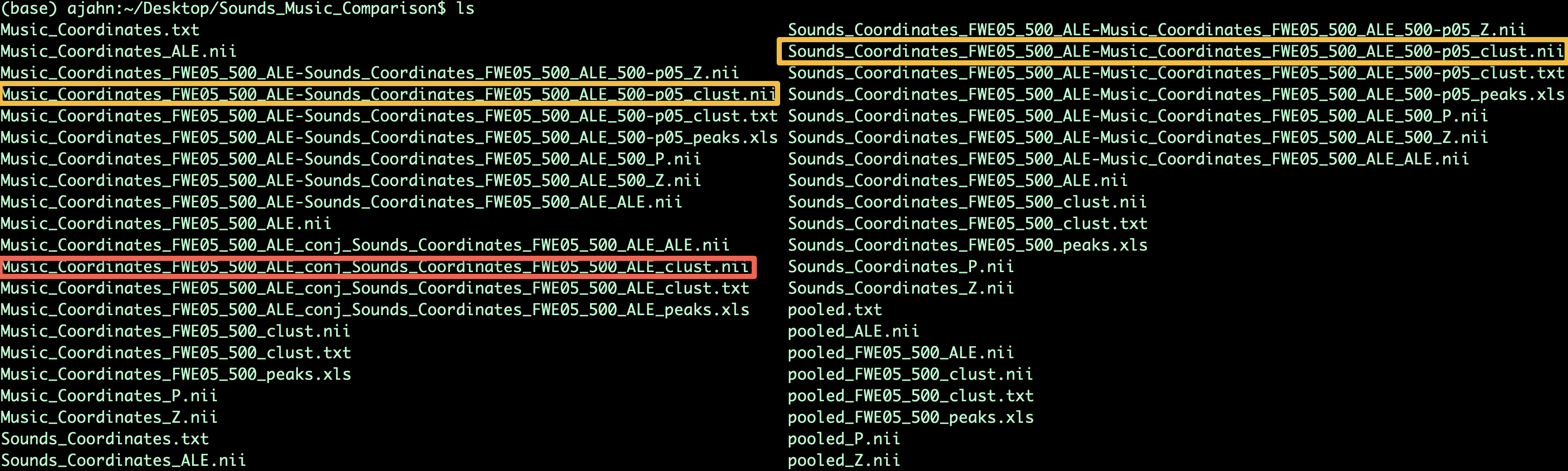
Output from the Contrast meta-analysis. The contrasts of Music-Sounds and Sounds-Music are highlighted in orange, while the conjunction between the meta-analysis maps is highlighted in red.
To view the results, load the output images in the MRI viewer of your choice, using an MNI template as an underlay. In this case, I will use AFNI to view the images, selecting the MNI152_2009_template.nii.gz template as an underlay and then loading the conjunction between the meta-analyses (i.e., Music_Coordinates_FWE05_500_ALE_conj_Sounds_Coordinates_FWE05_500_ALE_ALE.nii), which will display cluster-corrected ALE results for significant overlap between the meta-analysis maps. (The map Music_Coordinates_FWE05_500_ALE_conj_Sounds_Coordinates_FWE05_500_ALE_clust.nii, useful for visualizing how many clusters there are, displays the ALE results encoded with integers indicating which cluster a voxel belongs to, such as 1, 2, 3, etc.) You may find it useful to display the ALE results side-by-side with their accompanying text files; for example, the file Music_Coordinates_FWE05_500_ALE_conj_Sounds_Coordinates_FWE05_500_ALE_peaks.xls provides MNI coordinates for peaks within the cluster, the Activation Likelihood Estimate, and where the peaks are located according to an MNI atlas. For a more detailed, annotated summary, look in the file Music_Coordinates_FWE05_500_ALE_conj_Sounds_Coordinates_FWE05_500_ALE_clust.txt, which lists the cluster volume, peak ALE coordinate, and probabilistic atlas classifications of each cluster.
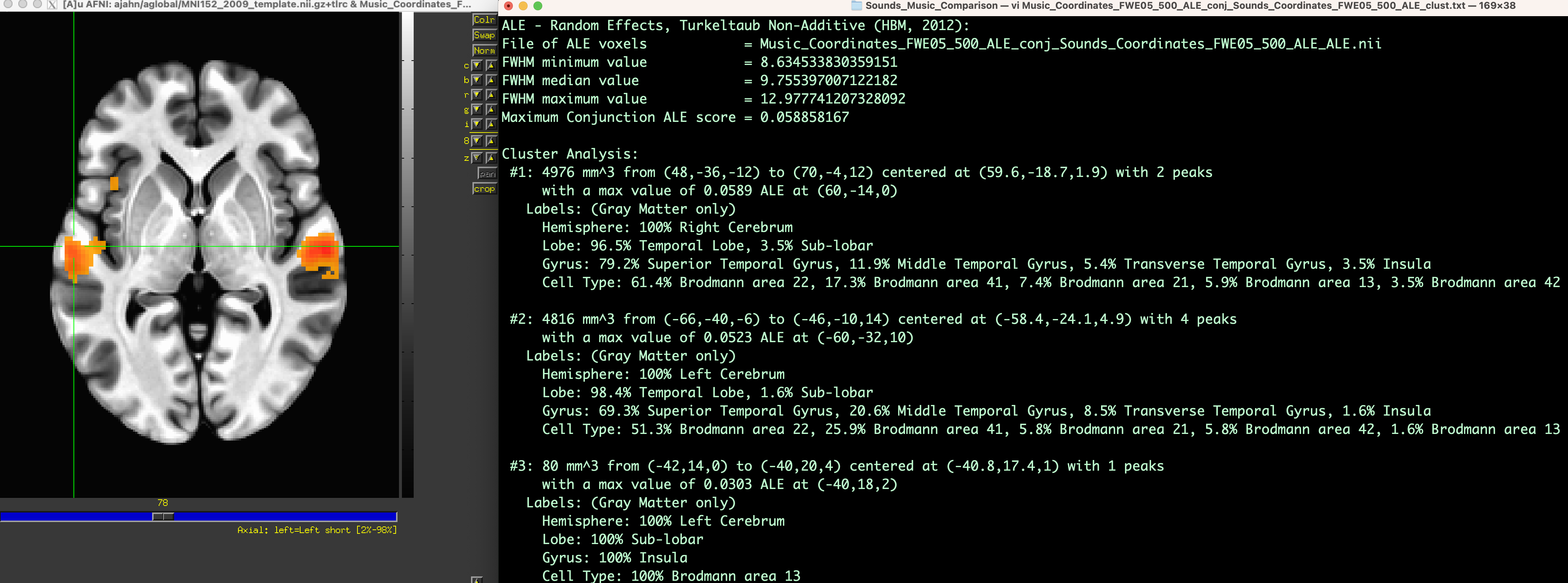
Example output from the Conjunction meta-analysis, displaying significant overlap between the meta-analysis maps for Music and Sounds. The panel on the left displays the cluster-thresholded conjunction map on an MNI template, and the panel on the right provides statistical and localization details for each cluster.
Next Steps
Now that you are familiar with one of the most popular meta-analysis packages, we will learn how to use another meta-analysis package called “Seed-Based D Mapping”. To learn more about how to use this package, click the Next button.