SPM Tutorial #8: Group Analysis
Overview
Our goal in analyzing this dataset is to generalize the results to the population that the sample was drawn from. In other words, if we see changes in brain activity in our sample, can we say that these changes would likely be seen in the population as well?
To test this, we will run a group-level analysis (also known as a second-level analysis). In SPM, this means that we calculate the standard error and the mean for a contrast estimate, and then test whether the average estimate is statistically significant. We will be doing this group-level analysis using a summary statistic approach which ignores the variability in the parameter estimates, and performs a t-test over the mean parameter estimates from each subject.
Specifying the 2nd-Level Analysis
Once all of the 1st-level analyses have finished, create a new directory in which to store your 2nd-level results. From the Matlab terminal, navigate to the Flanker directory containing all of your subjects, and type mkdir 2ndLevel_Inc-Con.
From the SPM GUI, click on the button Specify 2nd-level. The default test that will be conducted is a one-sample t-test, and there are only two fields that need to be filled in: The output directory for the results, and the scans that you will conduct the test on - in other words, the contrast images that were created during each 1st-level analysis.
Double-click on the Directory field, and select the 2ndLevel_Inc-Con folder you just created. For the Scans field, navigate to sub-01’s 1stLevel directory, and select the Incongruent-Congruent contrast image, con_0001.nii. Navigate into all of the other subject’s 1stLevel directories, and select the con_0001.nii image for each subject. The animation below shows a couple of ways to make this process quicker. When you have finished selecting the con_0001.nii image for all 26 subjects, click the green “Go” button.

Note
If you forget which contrast image corresponds to which conditions being contrasted, you can figure it out using one of the following methods. One option is to load the SPM.mat file through the Results GUI for a sample subject, and see which number contrast corresponds to the con images that are generated in each subject’s folder. The other way is to use the Matlab terminal to navigate to a sample subject’s 1stLevel results folder, and type load SPM.mat. This will load the SPM structure into memory, and this structure contains information about all of the data that was entered into the 1st-level analysis. If you then type SPM.xCon.name, Matlab will return the label for each contrast.
Estimating the 2nd-Level Analysis
Specifying the model will only take a second. When it has finished, you will need to estimate the model, just as you did with the 1st-level analyses. From the SPM GUI, click the Estimate button. Select the SPM.mat file from the 2ndLevel_Flanker directory that you created, and then click the green “Go” button.
Viewing the Results
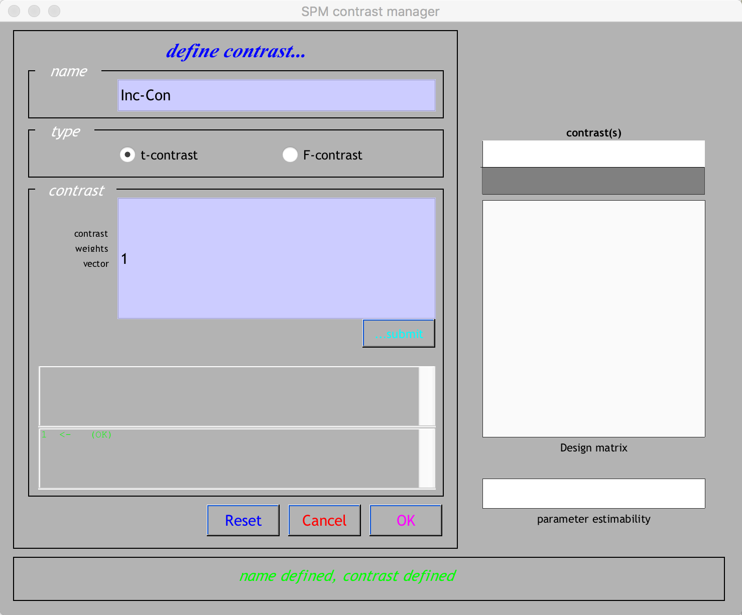
As with the 1st-level analyses, we can now view the results by clicking on the Results button from the SPM GUI. Select the SPM.mat file from the 2ndLevel_Inc-Con directory, and click Done. You will see another contrasts window, with a slight difference: Whereas the 1st-level analyses had a design matrix that contained all of the regressors in the model, this design matrix looks like a white box. That indicates that there is only one regressor to test, namely the mean activation across all of the individual contrast images that went into the model.
Click Define new contrast..., call the contrast “Inc-Con”, and give it a contrast weight of 1. When you are finished, it should look like this:
Click OK, and then click Done. You will be asked the same questions as before about masking, cluster-thresholding values, and cluster extent. For this group analysis, select the following:
apply masking -> none
p value adjustment to control -> none
threshold {T or p value} -> 0.001
& extent threshold {voxels} -> 20
This will threshold the image to only show clusters that are composed of individual voxels each passing a threshold of 0.001. Later, we will learn how to determine what cluster-defining threshold gives us a false positive rate of 0.05.
When you are finished, you should see output like this, showing a significant cluster in the dorsal medial prefrontal cortex:
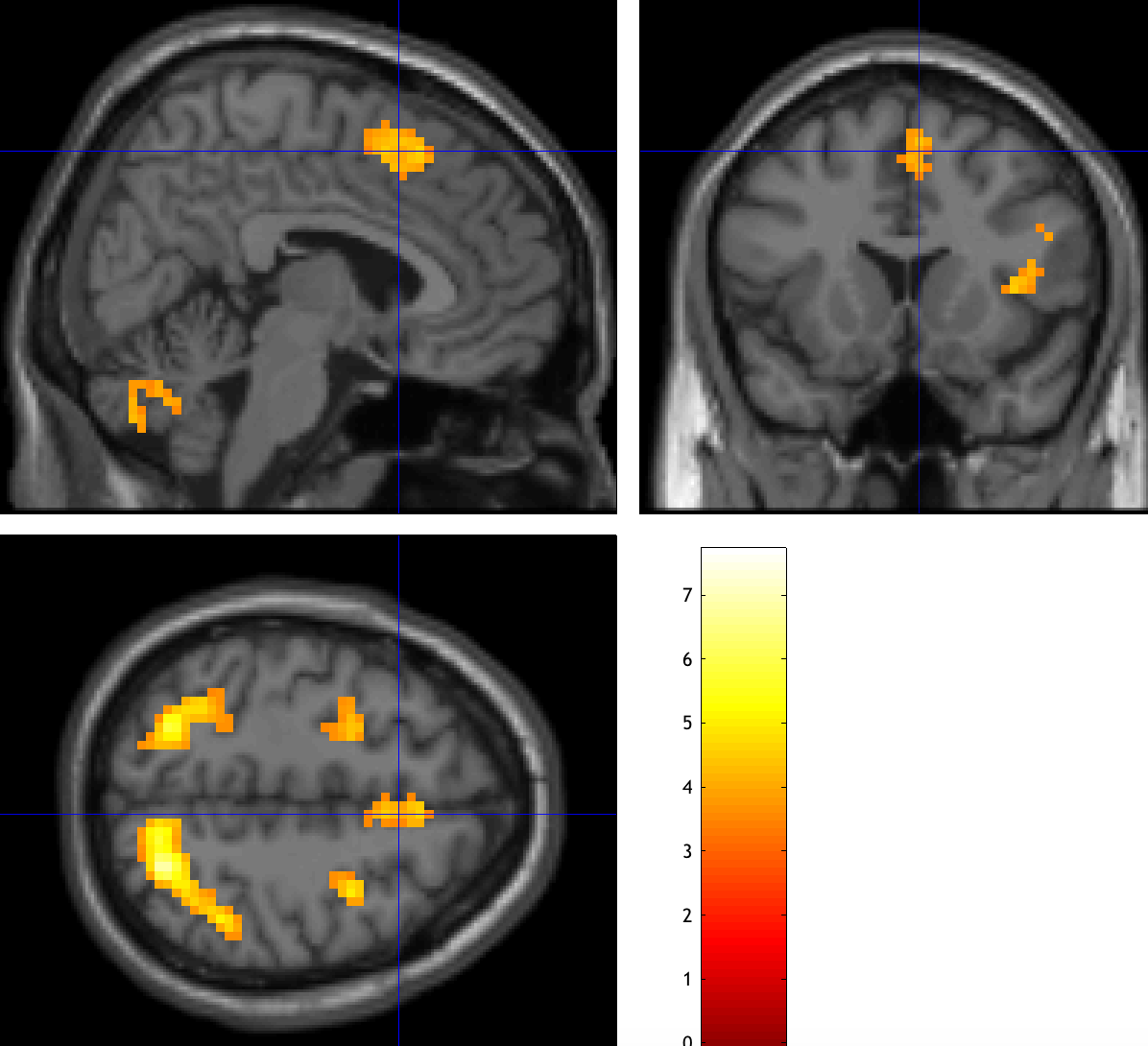
2nd-Level Results for Incongruent and Congruent
If you are only interested in where there are significant differences between the Incongruent and Congruent conditions, then the above steps are all that you need to do. As you will see in a later chapter on ROI Analysis, however, it is useful to examine the activity in each condition separately to see what drives the effect of Incongruent-Congruent.
To prepare for that analysis, navigate to the Flanker directory and create two new 2nd-level directories, one for the simple effect of each contrast:
mkdir 2ndLevel_Incongruent
mkdir 2ndLevel_Congruent
Using the same procedure above for determining which contrast is located in the SPM.mat file, we find out that the Incongruent contrasts are located in the con_0003.nii file for each subject, and the Congruent contrast are located in the con_0004.nii file for each subject. Starting with the Incongruent contrast images, click on the Specify 2nd-Level button on the SPM GUI, and for the Directory input, select the 2ndLevel_Incongruent folder. Using a similar method as above, select the con_0003.nii images for each subject. Estimate the model, and load the SPM.mat file into the Results GUI. Label the contrast Incongruent, and assign it a contrast weight of 1. Use the same options as you did for the Inc-Con contrast.
As an exercise, create a second-level result for the Congruent contrasts. If you examine the Incongruent and Congruent results at the same threshold, do you see what you would expect given the Inc-Con contrast that you viewed above?
Note
How can you determine what the cluster threshold needs to be in order to determine whether a cluster is significant? The table underneath the glass brain shows a list of clusters that pass the thresholds you specified, and the column pFWE-corr displays the p-value associated with that cluster (“cluster-level”) or individual voxel (“peak-level”). In other words, any clusters that have a corresponding pFWE-corr value of 0.05 or less can be considered statistically significant.
The actual threshold for determining the p=0.05 cluster threshold is at the very bottom of the table, next to the string FWEc:. Write down the number in that field, and then rerun your Results using that threshold. The clusters that remain should all be statistically significant.
For alternative methods of estimating a cluster threshold, see Appendix A, specifically the section “SPM’s Cluster Correction”.
When you have finished creating all of the second-level analyses, try the remaining exercises to test your understanding of what you have just learned.
Exercises
Display the results on one of the MNI template brains using the “sections” option. Make the table show only the cluster in the dorsal medial prefrontal cortex (roughly the coordinates 5, 20, 50) by navigating to those coordinates and clicking “current cluster.” Take a snapshot of those results.
Go back to the Results GUI, and create a contrast that tests for voxels showing significant activation for Congruent-Incongruent. Use an uncorrected p-threshold of 0.05 and a cluster extent threshold of 20, display the results on a template brain, go to coordinates 0 32 1, and take a snapshot of your results.
Video
For a video overview of group-level analysis, click here.