Appendix B: Psychophysiological Interactions (PPI) in SPM¶

Note

This page is currently where I am jotting down notes for how to do a group-level PPI in SPM.

Download¶

Data is from the Human Connectome Project database; click on the dropdown menu next to WU-Minn HCP Data - 1200 subjects and select subjects with 3T MR Session Data.

Data Structure¶

Within each subject directory (with subject IDs like 100206), there is a directory called MNINonLinear/Results. This contains 2 directories with functional data, tfMRI_SOCIAL_LR and tfMRI_SOCIAL_RL. The data have been preprocessed, except for the smoothing step; you will need to apply that yourself.

Before you begin, create the following directories in each subject’s folder with Matlab’s mkdir command:

1stLevel_Concat
PPI

Preparing for the PPI Analysis¶

Once the data have been smoothed, the directories will contain files called “stfMRI_SOCIAL_LR.nii” and “stfMRI_SOCIAL_RL.nii”. We will be combining these into a single dataset, because SPM’s PPI function cannot process datasets with more than one run. To account for the fact that we are combining all of the data into one run, and that the signal may be systematically different in one run compared to another, we will be including both in our 1st level analysis.

Concatenating the Movement Regressors¶

The movement regressors will also need to be vertically concatenated into a single file. Navigate into the tfMRI_SOCIAL_LR directory and type:

cat Movement_Regressors.txt ../tfMRI_SOCIAL_RL/Movement_Regressors.txt > allMovement_Regressors.txt

Creating the Model Specification Batch¶

In this study, the TR is 0.72, and each run has 274 volumes. That means that each run is 0.72 * 274 = 197.28 seconds long. We will therefore add 197.28 to the second run’s timings to generate the following onset times for a single concatenated run:

Mental: 8.21 122.056 205.476 243.287 319.336

Rnd: 46.008 84.032 160.081 281.311 357.36

Each onset time lasts for 23 seconds (i.e., this is a block design). There may be discrepancies of a few thousandth of a millisecond between subjects, but since it is a block design, this timing scheme can be used for every subject.

Now open the SPM GUI, click on Batch, and from the menu click on SPM -> Stats -> fMRI model specification. Add the following modules, also in the SPM -> Stats menu: Model estimation and Contrast Manager.

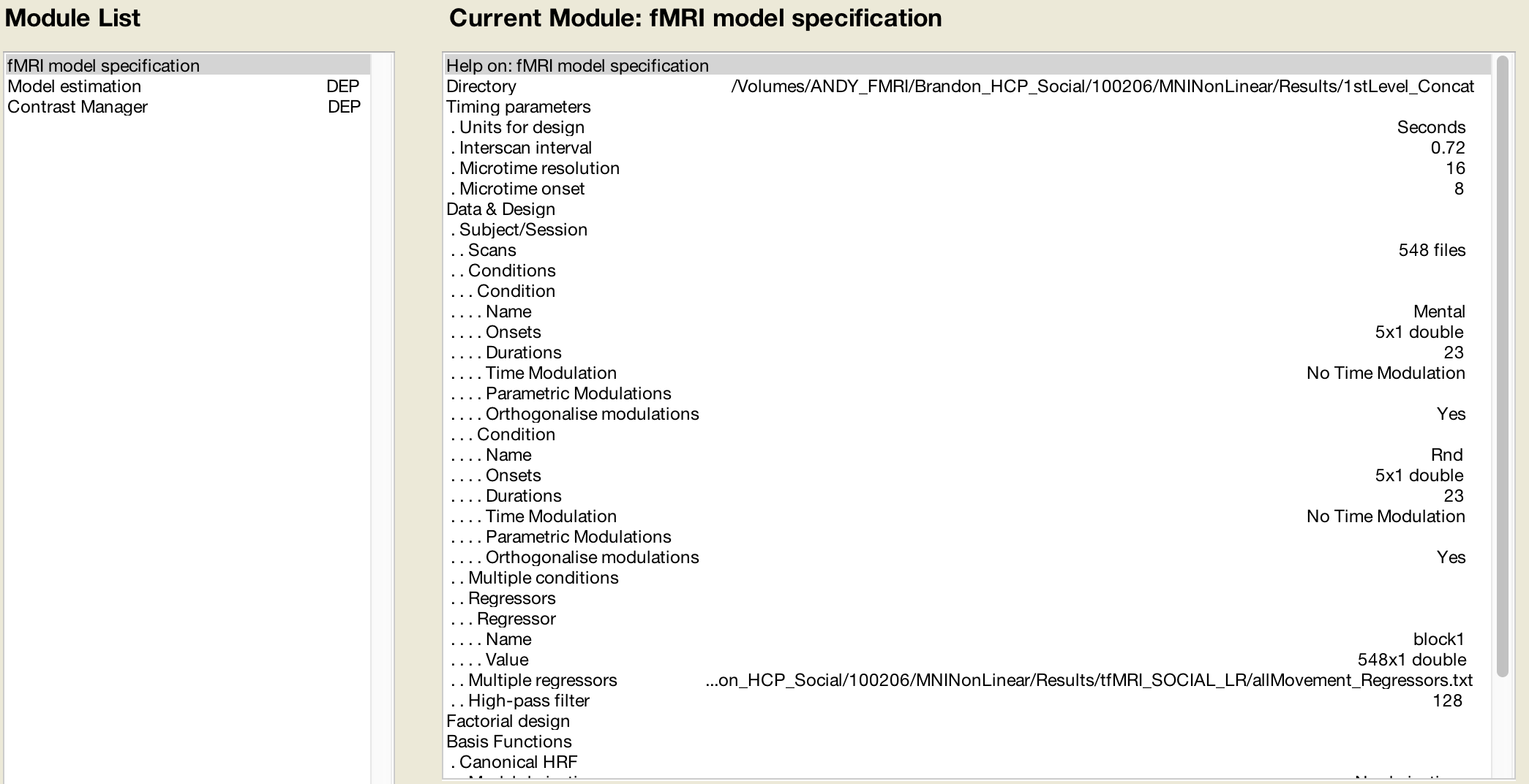
In the fMRI model specification module, select the 1stLevel_Concat folder as the Directory. Change the Units for design to Seconds, and the Interscan interval to 0.72. Click on Data & Design and then select New: Subject/Session. Double-click on the Scans button, and select the stfMRI_SOCIAL_LR.nii files first, and then the stfMRI_SOCIAL_RL.nii files (this order is important). In the selection window, enter ^s.* in the Filter field to only view those files beginning with an ‘s’, and in the Frames field type 1:274 to expand the number of volumes to 274. Do this for each of the LR and RL directories.

Now click on Conditions, and click twice on New:Condition. Rename the first condition Mental, and the second condition Rnd. Specify a duration of 23 for both, and in the Onsets field, copy and paste the above timings for each corresponding condition.

To account for the effect of block, click on Regressors, and select New: Regressor. Set the Name to block1, and then double-click on Value. In the Value field, type the following:

kron([1 0]',ones(274,1))

Which will create a column vector with 274 ones, followed by 274 zeros. These represent the first block and the second block, respectively.

Finally, click on Multiple regressors, and load the allMovement_Regressors.txt file that you created above. When you have finished, your model specification should look like this:

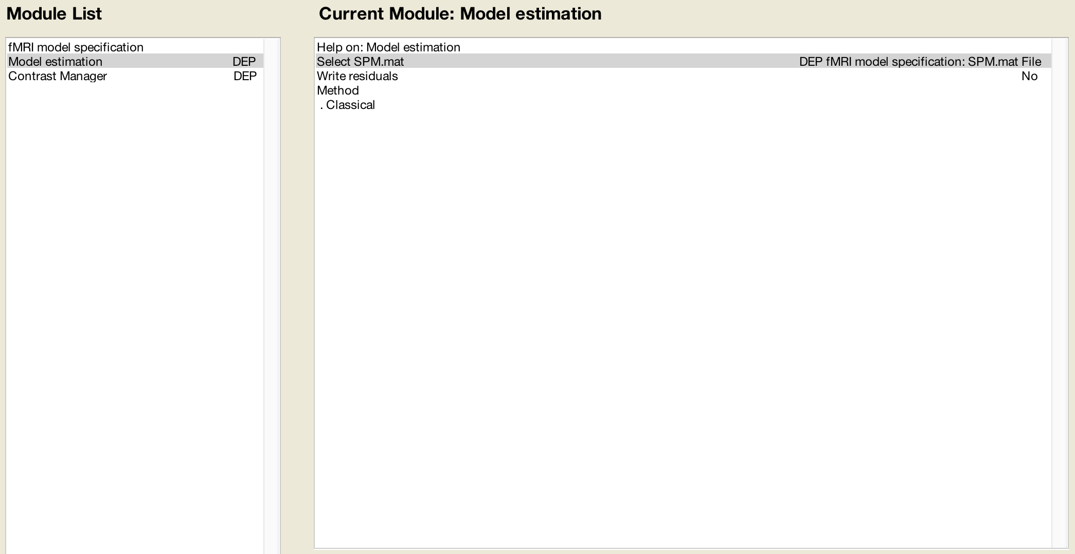
../../_images/SPM_PPI_ModelSpecification.png

Now we will finish editing the other modules in our batch. Click on Model estimation in the lefthand window, highlight Select SPM.mat with your mouse, and then click on Dependency. Choose the SPM.mat file from the fMRI model specification step.

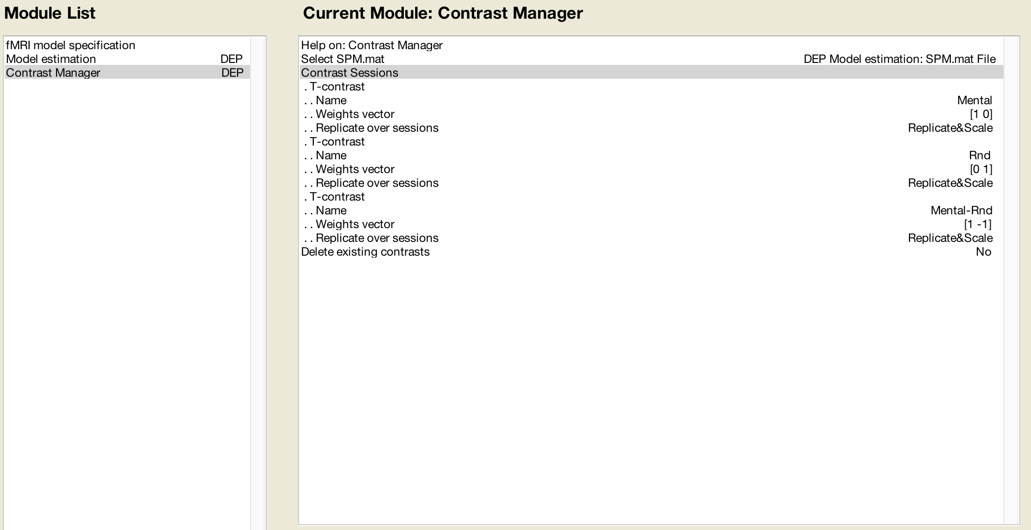
../../_images/SPM_PPI_ModelEstimation.png

Next, click on the Contrast Manager module. Again, highlight Select SPM.mat with your mouse, and then click on Dependency. Choose the SPM.mat file from the model estimation step. Then click on Contrast Sessions and click on New: T-contrast to create three new T-contrasts. Label the first one Mental, the second one Rnd, and the third one Mental-Rnd. For the Mental contrast, specify a vector of [1 0]; for the Rnd contrast, specify a vector of [0 1]. For the Mental-Rnd contrast, specify a vector of [1 -1]. Since there is only one run, you do not need to Replicate&Scale the contrast weights, but doing so won’t affect your analysis either.

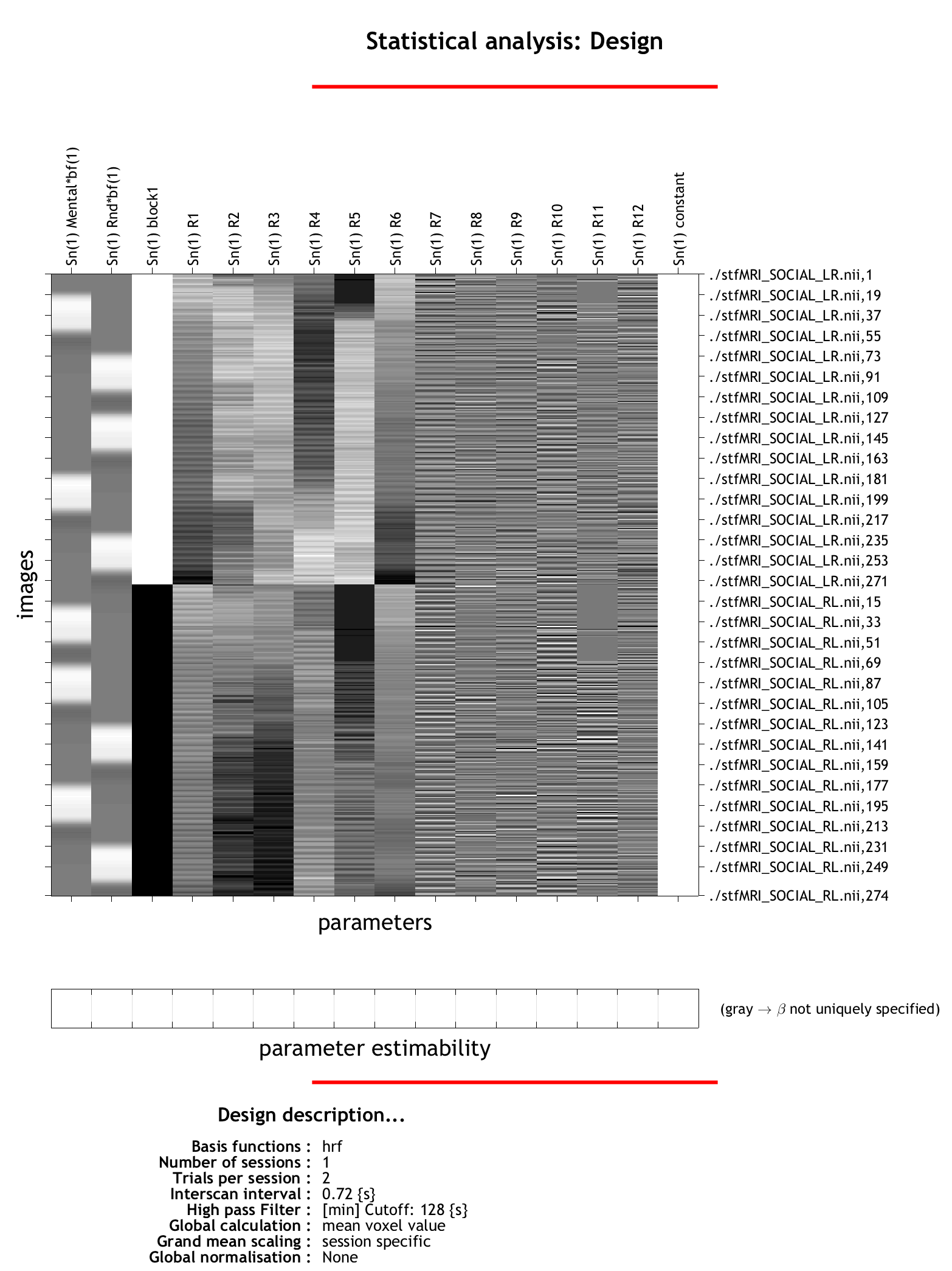
../../_images/SPM_PPI_ContrastManager.png

Now save the batch and script by clicking on File -> Save Batch and Script. Label the output Sample_Concatenated_1stLevel. Then click on the green “Play” button in the top left corner of the GUI to run the batch. It should take about 15-20 minutes. When it has finished, the design matrix should look like the following:

The PPI Interface¶

We are now ready to begin our PPI analysis. Before you start, make sure that you have a region of interest (or ROI, also known as a mask) to use. These can be created either using Marsbar or another software package, such as AFNI’s 3dUndump or FSL’s fslmaths. In our example, assume you’ve created an ROI called dmPFC that is centered within the dorsomedial prefrontal cortex. These ROIs will be stored in the directory that contains all of the subject directories.

To begin, open the SPM GUI and click on the PPIs button. You will be prompted to select an SPM.mat file; select the one you just created that is located in the 1stLevel_Concat directory. You will then be prompted to select an analysis type; choose psychophysiologic interaction and then select VOI_dmPFC.mat. Include Mental and Rnd when prompted, and assign them weights of 1 and -1, respectively. Label the output PPI as PPI.

You will then see a window showing the hemodynamic and estimated neuronal responses (after the hemodynamic response has been deconvolved), and the onset times of the blocks of your experiment, convolved with the HRF.

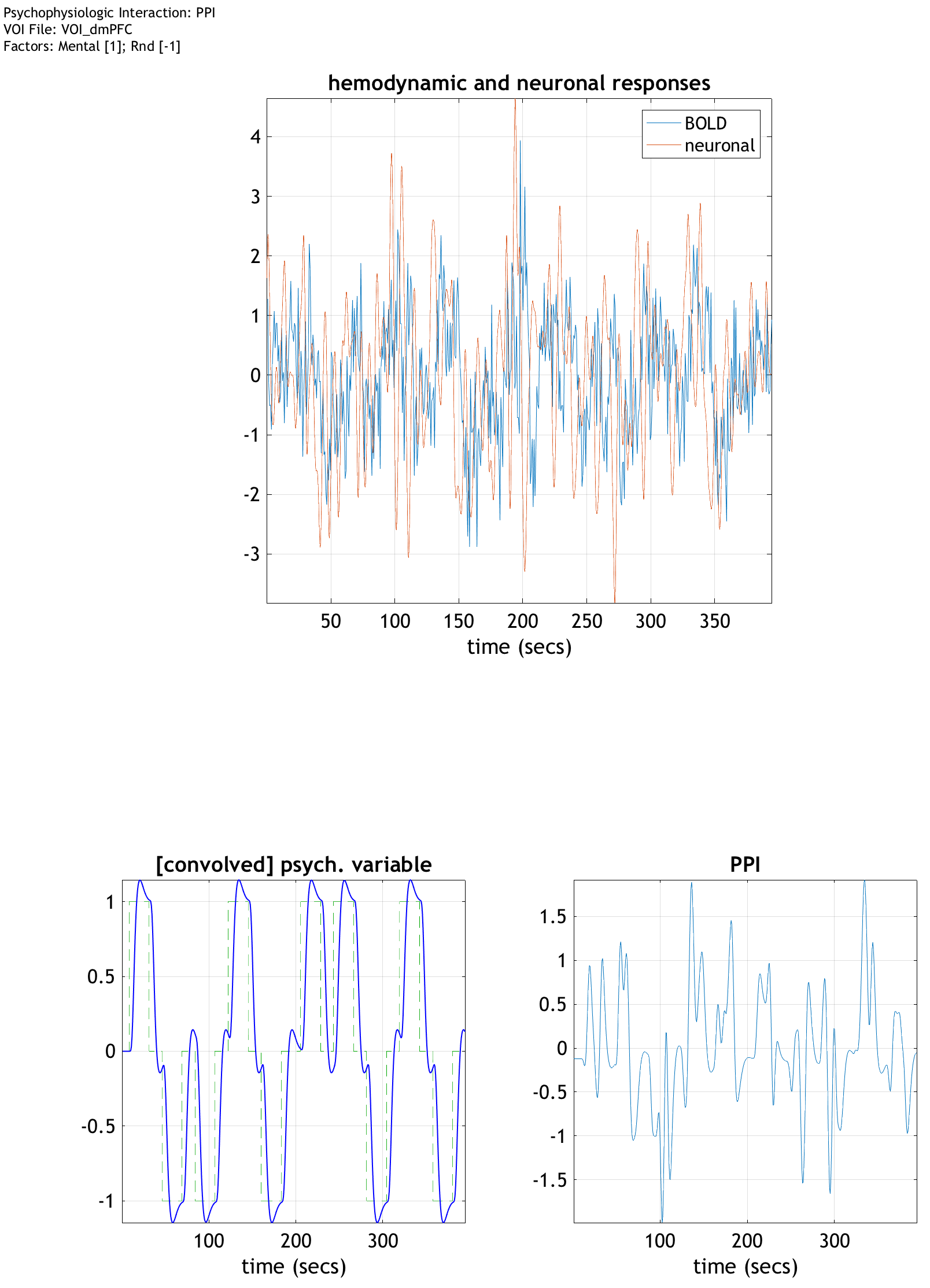
This will create a variable in your workspace called PPI. You can load it from the command line by typing load PPI. This enables the use of several fields of the PPI variable, including:

PPI.P: The convolved onset times
PPI.Y: The time-series extracted from the VOI
PPI.ppi: The Interaction term created by the PPI analysis

Our goal is to now include these three variables in another GLM, which will allow us to estimate a beta weight at each voxel for the PPI using a VOI (in this case, the dmPFC).

Setting up the PPI Analysis¶

First, enable the use of the PPI fields by typing the following at the Matlab prompt:

load PPI_PPI.mat

You should see the variable PPI in your workspace.

Now, open the SPM GUI and click the Batch button. As before, from the menu click on SPM -> Stats -> fMRI model specification. Add the following modules, also in the SPM -> Stats menu: Model estimation and Contrast Manager.

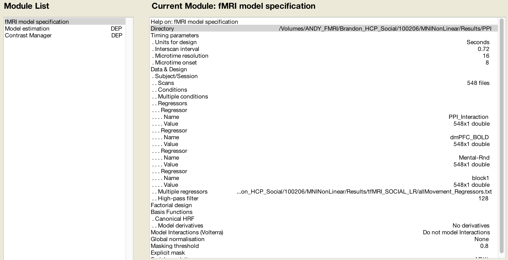
In the fMRI model specification module, set up the model as previously: Units of Time in Seconds and TR of 0.72, and the same Scans as before. Select the folder PPI as the output directory. Then click on Data & Design, and click on New: Subject/Session. Instead of conditions, however, this time we will enter Regressors, since they have already been convolved with the hemodynamic response function. Create 4 new Regressors, and give them the following names and values:

Regressor 1: Name=PPI_Interaction / Value=PPI.ppi
Regressor 2: Name=dmPFC_BOLD / Value=PPI.Y
Regressor 3: Name=Mental-Rnd / Value=PPI.P
Regressor 4: Name=block1 / Value=kron([1 0]',ones(274,1))

Also double-click on Multiple regressors and specify the allMovement_Regressors.txt file. When you are finished, the model specification window should look like this:

../../_images/SPM_PPI_Model_Specification_PPI.png

Set the Model estimation SPM file to a dependency calling upon the output from the fMRI model specification module, and specify the SPM file in the Contrast manager as the dependency output from the Model estimation module. In the Contrast Manager module, create one T-contrast, and give it the name dmPFC_PPI_Interaction. Give it a weight vector of 1. Then save the batch and script as Run_dmPFC_PPI in the results directory which contains the 1stLevel_Concat and PPI folders. Then press the green “play” button to run the analysis.