Appendix F: Parametric Modulation
Overview
This appendix demonstrates how to set up a parametric modulation analysis in FSL. An overview of what parametric modulation is can be found here, along with code for downloading the data. If you already have Amazon Web Services installed, then you can open a Terminal and type the following:
aws s3 sync --no-sign-request s3://openneuro.org/ds000005 ds000005-download/
mv ~/Downloads/ds000005-download ~/Desktop/Gambles
This will create a new folder on your Desktop called Gambles, which we will use to store the data and the output from our analyses.
Preprocessing the Data
To prepare the data for a parametric modulation analysis, we will create a preprocessing pipeline similar to the one we used for the example dataset here. If you haven’t already, go through the tutorial with the Flanker dataset; there you can find the details of each preprocessing and statistical analysis step, which we won’t discuss here in depth.
Creating the Timing Files
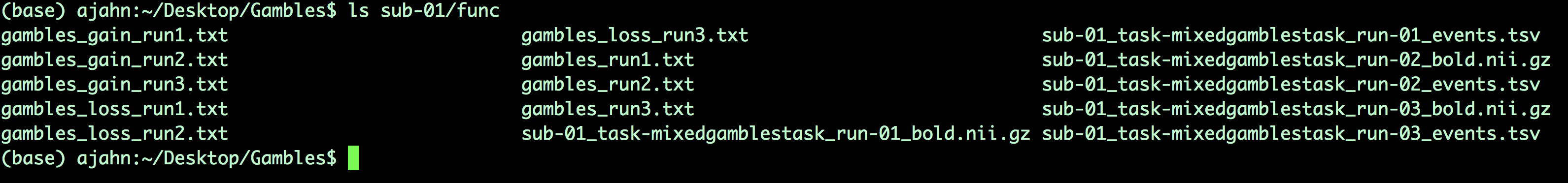
We will first create timing files that contain onsets for the Gamble, the parametric value for the potential Gain, and the parametric value for the potential Loss, for each run; in total, we will create nine regressors.
You can download a script to convert the timings into a format that FSL understands by clicking here, clicking on the Raw button, and right-clicking anywhere on the screen and selecting Save As. Save the file as a shell script into the Gambles directory. Once it has been downloaded, navigate to that directory with a Terminal and run the script by typing bash make_FSL_Timings_Gambles.sh. You should see nine text files in each func directory:
Skull-Stripping the Brain
Before we open the FEAT GUI, we need to skull-strip the brain using bet2. From the Gambles directory, navigate to the sub-01 directory and type the following:
bet2 anat/sub-01_T1w.nii.gz anat/sub-01_T1w_brain.nii.gz
Setting up the FEAT GUI
Now open the FEAT GUI by typing Feat_gui from the Terminal. Just as in the FSL tutorial, we will create a template design file that we can use in a for-loop to analyze all of the subjects.
In the Data tab, click on Select 4D data and navigate to the func folder; select the file sub-01_task-mixedgamblestask_run-01_bold.nii.gz and click OK. In the Output directory field, type run1.
Leave the defaults as they are in the Pre-stats tab. In the Registration tab, select the file in the anat directory, sub-01_T1w_brain.nii.gz. The search space is up to you, but to speed up the analysis, change Normal Search to Full Search for both the main structural image and the standard space image, and select 12 DOF for both of them as well.
In the Stats tab, click on Full Model Setup. Type the number 3 in the field Number of original EVs, and label them in the following order:
Gambles
Gain_PM
Loss_PM
For each one, select Custom (3 column format) for the Basic Shape, and select the corresponding filename; e.g.,
Gambles -> gambles_run1.txt
Gain_PM -> gambles_gain_run1.txt
Loss_PM -> gambles_loss_run1.txt
In the Contrasts & F-tests tab, create 4 contrasts, and label them as follows with the corresponding contrast weights:
Gambles [1 0 0]
Gain_PM [0 1 0]
Loss_PM [0 0 1]
Gain-Loss_PM [0 1 -1]
When you are done, click on the Save button at the bottom of the GUI, and call it design_run1.fsf. Save it in the Gambles directory. Do the same procedure for the other two runs, updating the functional run and the timing files, and saving the design files as design_run2.fsf and design_run3.fsf. Save these files into the Gambles directory as well.
Next, download the file run_1stLevel_Analysis_Gambles.sh, saving it into the Gambles directory just like you did with the timing conversion script. Run it by typing:
bash run_1stLevel_Analysis_Gambles.sh
You should see an HTML file open for each run that is analyzed, which will generate 48 tabs total. The entire analysis should take four or five hours, depending on the speed of your machine.
Higher-Level Analysis
Setting up the Second-Level Analysis
From the Gambles directory, type:
ls -d $PWD/sub-??/run*
This will create a list of all of the first-level FEAT directories. Copy the output to your clipboard, and open up a new FEAT GUI. Select Higher-level analysis from the dropdown menu, and make sure that Inputs are lower-level FEAT directories is selected. Change the Number of inputs to 48, and then click on Select FEAT directories. Click Paste, and then press ctrl+y on the keyboard to paste the list of FEAT directories. Click OK, and leave the boxes checked next to Use lower-level copes. For the Output directory, enter Gambles_2ndLevel.
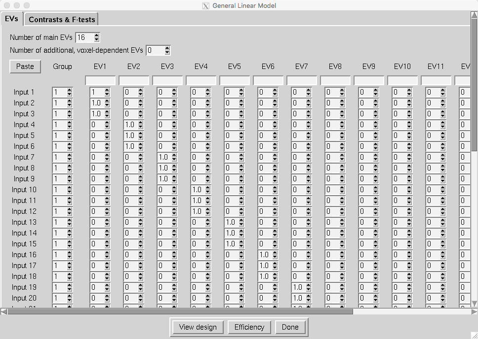
In the Stats tab, change the Mixed effects to Fixed effects. Click on Full Model Setup. Change the Number of main EVs to 16, and fill in the matrix with three 1’s for each subject, as in the following figure:
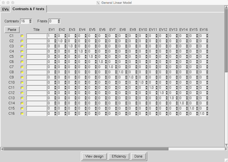
And update the Contrasts & F-tests tab so that there are 16 contrasts, and a contrast weight of 1 per subject:
Click OK, and then click the Go button. This will average the parameter estimate for each regressor across all three runs, and it will take an hour or two.
Setting up the Third-Level Analysis
Open a new FEAT GUI, and select Inputs are 3D cope images from FEAT directories from the dropdown menu. Change the Number of inputs to 16, and set the Output directory to Gambles_3rdLevel_Gain. Use a Terminal to navigate to the directory Gambles_2ndLevel.gfeat/cope2.feat/stats, and type:
ls $PWD/cope* | sort -V
This will return a list of all of the cope images for the second contrast we specified, which is the parametric modulation of Gain. Copy this list, click on Select cope images, click Paste, and then type ctrl+y to paste the list. Click OK.
In the Stats tab, you can leave the default of Mixed effects: FLAME 1. Click on Model setup wizard, and select single group average. Click Process, and then click Go. This analysis will take ten to twenty minutes.
Viewing the Results
To view the results, navigate to the directory Gambles_3rdLevel_Gain.gfeat and open fsleyes. Select File -> Add Standard and choose the template MNI152_T1_1mm. Next, click on File -> Add from file, and select thresh_zstat1. Change the colorscale to Red-Yellow to better see the outline of the cluster, and click on the Gear icon and choose Linear interpolation to smooth the edges. You should see something like this:
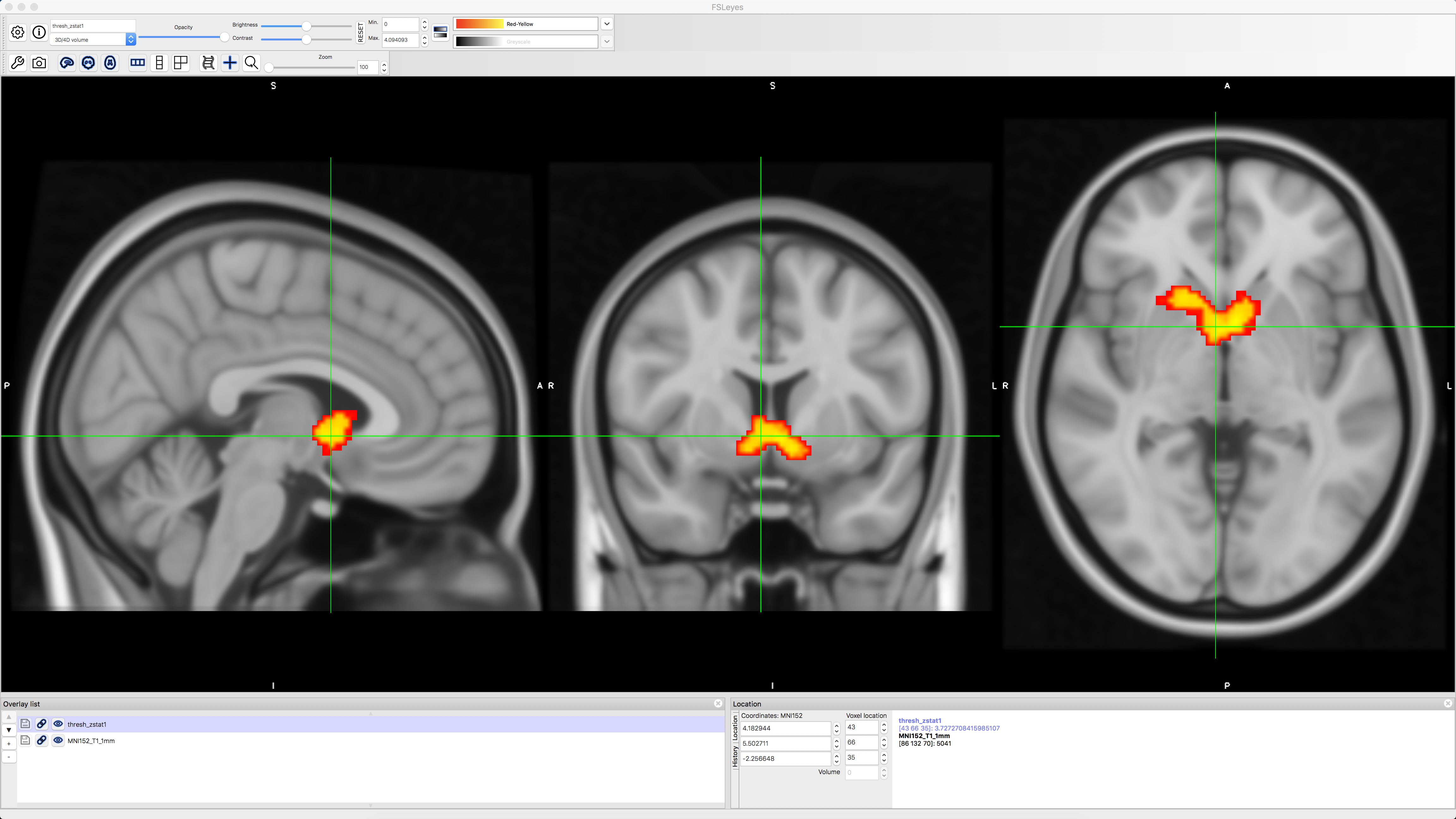
We see that there is significant parametric modulation of Gain within the ventral striatum, as we would expect. However, we also know that FSL’s FLAME1 method for cluster correction can be overly conservative; see, for example, Figure 1 of Eklund et al., 2016. We can instead use a non-parametric option such as randomise in conjunction with threshold-free cluster enhancement, in order to balance the width and the height of each cluster. This will strike a balance between false positives and false negatives; our false positive rate will be kept to 5%, but we will also see cluster that we wouldn’t otherwise with traditional cluster correction methods.
To do this, navigate to the directory Gambles_2ndLevel.gfeat/cope2.feat/stats, which contains the z-statistic images for the parametric modulation of Gain. Merge the files into a single dataset, and move it to the main Gambles directory:
fslmerge -t allZs.nii.gz zstat*
mv allZs.nii.gz ../../..
cd ../../..
Now run randomise, using the -1 flag to indicate that it is a one-sample t-test, and the -T flag to do threshold-free cluster enhancement (TFCE). We will run 5000 simulations:
randomise -i allZs.nii.gz -o allZs_randomise -1 -T -n 5000
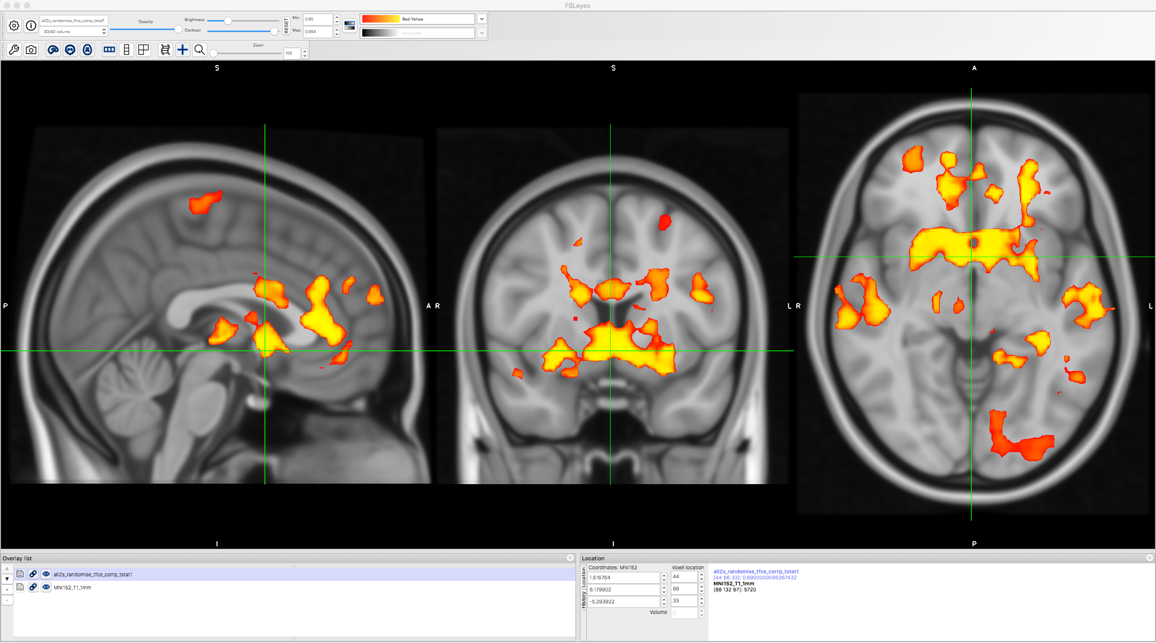
Load the file allZs_randomise_tfce_corrp_tstat1 in fsleyes, and change the Min. threshold of 0.95. This will show all of the TFCE clusters at an alpha threshold of p=0.05. Note how many more clusters there are, and how these were hidden with the FLAME1 approach.
Next Steps
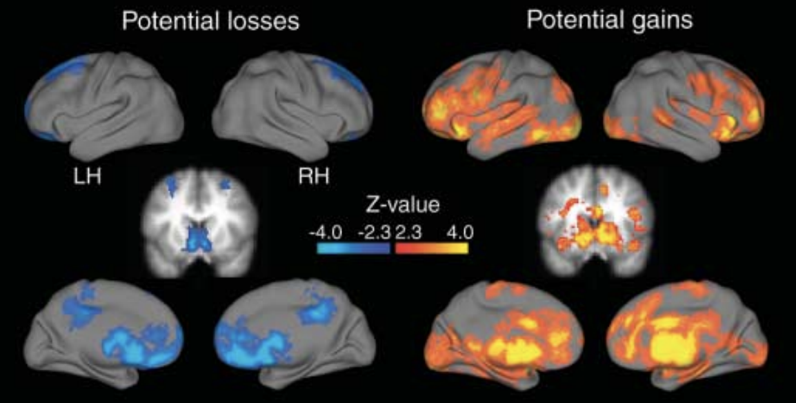
As an exercise, try running the same analysis with the parametric modulation of Loss; these are located in the 2ndLevels directory as cope3. You may have to look at the unthresholded results, since in my experience the Loss results do not pass the threshold in either FLAME1 or TFCE. Nevertheless, you should still see an association of negative BOLD signal with the Loss parametric modulators. Compare your results to those of Tom et al., 2007:
Video
A video demonstration of how to analyze the Tom et al. 2007 dataset can be found here.