Appendix B: Analyzing Rat Data
Overview
In addition to analyzing human brains, AFNI can be used to analyze animal brains as well. In this tutorial, we will replicate the results of a recent Nature paper published by Sirmpilatze, Baudewig, & Boretius (2019); a link to the paper can be found here, and a link to the data on OpenNeuro can be found here.
The aim of the study was to examine how fMRI measures from task-based and resting-state analysis change over time when rats are anesthetized with Medetomidine. For our purposes, we will simply replicate the task-based effects of electrical forepaw stimulation (or EFS), as well as the resting-state results. The advanced user may choose to replicate their temporal variability analyses, but that is beyond the scoope of the current tutorial.
Preprocessing the Data
The Methods section of the paper states that the data were analyzed using Python tools, which called upon a combination of FSL and AFNI commands; nevertheless, we will use mostly AFNI commands here, as well as an advanced registration tool called ANTs. In particular, we will replicate the following preprocessing steps were done:
Slice-timing correction;
Band-pass filtering of less than 0.01Hz and greater than 0.15Hz;
Spatial smoothing of 0.5mm.
Coregistration between the functional and structural images;
Note that in this study motion correction was not performed, since the rats were anesthetized and did not move much. Consequently, motion regressors were not used in the model.
Let’s begin with slice-timing correction. Using 3dinfo on the first EFS run, we can see the following the in the header:
Dataset File:    sub-01_task-efs_run-01_bold.nii.gz
Identifier Code: NII_GMnEUUfC2G6z4SOYguib2A  Creation Date: Tue Apr 18 12:27:02 2023
Template Space:  ORIG
Dataset Type:    Echo Planar (-epan)
Byte Order:      LSB_FIRST {assumed} [this CPU native = LSB_FIRST]
Storage Mode:    NIFTI
Storage Space:   324,403,200 (324 million) bytes
Geometry String: "MATRIX(0.2,0,0,-12.8,0,-0.2,0,9.4,0,0,0.5,-5.94792):128,96,30"
Data Axes Tilt:  Plumb
Data Axes Orientation:
  first  (x) = Right-to-Left
  second (y) = Posterior-to-Anterior
  third  (z) = Inferior-to-Superior   [-orient RPI]
R-to-L extent:   -12.800 [R] -to-    12.600 [L] -step-     0.200 mm [128 voxels]
A-to-P extent:    -9.600 [A] -to-     9.400 [P] -step-     0.200 mm [ 96 voxels]
I-to-S extent:    -5.948 [I] -to-     8.552 [S] -step-     0.500 mm [ 30 voxels]
Number of time steps = 220  Time step = 1.50000s  Origin = 0.00000s
  -- At sub-brick #0 '?' datum type is float
  -- At sub-brick #1 '?' datum type is float
  -- At sub-brick #2 '?' datum type is float
** For info on all 220 sub-bricks, use '3dinfo -verb' **
The TR is 1.5s, there are 220 volumes in this run, and the voxel resolution is 0.2x0.2x0.5mm, which explains why the resolution in the sagittal and coronal planes looks lower than in the axial plane.
To slice-time correct this data, type:
3dTshift -tzero 0 -quintic -prefix sub-01_run-01_STC.nii sub-01_task-efs_run-01_bold.nii.gz
Next, we bandpass the data using 3dBandPass:
3dBandpass -prefix sub-01_run-01_STC_BP.nii 0.01 0.15 sub-01_run-01_STC.nii
And then smooth the data with a 0.5mm kernel:
3dmerge -1blur_fwhm 0.5 -doall -prefix sub-01_run-01_STC_BP_Smoothed.nii sub-01_run-01_STC_BP.nii
Note
On my machine, 3dBandpass appears to generate noisy output, regardless of the parameters used. For the rest of this tutorial, we will skip bandpassing by typing 3dmerge -1blur_fwhm 0.5 -doall -prefix sub-01_run-01_STC_Smoothed.nii sub-01_run-01_STC.nii.
First-Level Analysis
Looking within the task-efs_events.tsv file, we find that the onsets were:
onset   duration
60      30
150     30
240     30
This is the same for all of the subjects in the study, except for subject sub-07 (see note on the OpenNeuro repository). Accordingly, we can make an onset times file called Timings.txt, which contains this line of code:
60 150 240
Additional lines identical to the one above can be added for however many runs you are analyzing from this particular rat. However, since electrical forepaw stimulation should elicit a strong BOLD response, we should see a significant effect in just one run.
Once we have the timing file, we can insert it into a 3dDeconvolve command, such as the one below:
3dDeconvolve -input sub-01_run-01_STC_Smoothed.nii \
      -polort 3 \
      -num_stimts 1 \
      -stim_times 1 Timings.txt  'BLOCK(30,1)' \
      -stim_label 1 EFS \
      -gltsym 'SYM: EFS' \
      -glt_label 1 EFS \
      -tout -x1D X.xmat.1D -xjpeg X.jpg \
      -bucket stats.sub-01.nii
This will apply a 3rd-order polynomial (recommended for runs of 300s or more, which applies to this run), and convolves a 30-second boxcar basis function with each onset time specified in the Timings.txt file. The lines of code beginning with stim and glt specify the label for the output statistic dataset, and any contrasts. In this case, since there is only one condition, we are just doing a simple effect of electrical forepaw stimulation. Since the right forepaw was stimulated, the result should localize to the left somatosensory cortex. Once we run 3dDeconvolve and generate the dataset stats.sub-01.nii, we can load it into the AFNI viewer and overlay it on the T2-weighted anatomical image:
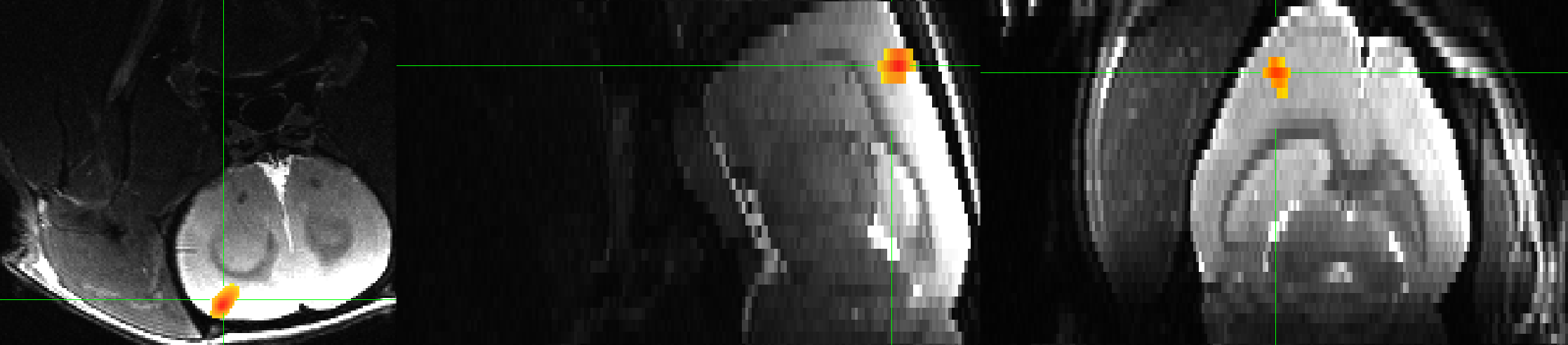
Single-rat results for a simple effect of electrical forepaw stimulation, thresholded at p=0.001, cluster threshold of k=40 voxels. Note that on these images, left is located on the left side of the panel, and the top of the brain is at the bottom of the image. We will later see how to reorient these images so that they match better with the figures reported in Sirmpilatze et al., 2019.
We can script this for all of the rats by navigating to the main directory containing the subjects and then typing:
echo "60 150 240" > Timings.txt
for i in sub-01 sub-02 sub-03; do
cp Timings.txt ${i}/func;
cd ${i}/func;
3dTshift -tzero 0 -quintic -prefix ${i}_run-01_STC.nii ${i}_task-efs_run-01_bold.nii.gz;
3dmerge -1blur_fwhm 0.5 -doall -prefix ${i}_run-01_STC_Smoothed.nii ${i}_run-01_STC.nii;
3dDeconvolve -input ${i}_run-01_STC_Smoothed.nii \
      -polort 3 \
      -num_stimts 1 \
      -stim_times 1 Timings.txt  'BLOCK(30,1)' \
      -stim_label 1 EFS \
      -gltsym 'SYM: EFS' \
      -glt_label 1 EFS \
      -tout -x1D X.xmat.1D -xjpeg X.jpg \
      -bucket stats.${i}.nii
 cd ../..
 done
Normalizing the Brains
Although there are rat templates available (such as the SIGMA template, available here, or the Waxholm Rat Atlas, available from the AFNI site), you may instead decide to use a study-specific template generated from the subjects included in your sample. For example, if we have six rats, we can choose one of them to be a fixed template image, and register all of the other rat brains to that image.
This was the approach used by the authors of the study, and they used a suite of normalization tools called Advanced Normalization Tools, or ANTs. Instructions for how to download and install the package can be found on the e-book here.
Once you have installed the package, let’s use the first six rat brains in the dataset. Using the first rat as the template, or fixed image, we can register the others to it by using the antsRegistrationSynQuick.sh command:
#!/bin/bash

antsRegistrationSyNQuick.sh -d 3 -f sub-01/anat/sub-01_T2w.nii.gz -m sub-02/anat/sub-02_T2w.nii.gz -o sub-02/anat/sub-02_to_sub-01
antsRegistrationSyNQuick.sh -d 3 -f sub-01/anat/sub-01_T2w.nii.gz -m sub-03/anat/sub-03_T2w.nii.gz -o sub-03/anat/sub-03_to_sub-01
antsRegistrationSyNQuick.sh -d 3 -f sub-01/anat/sub-01_T2w.nii.gz -m sub-04/anat/sub-04_T2w.nii.gz -o sub-04/anat/sub-04_to_sub-01
antsRegistrationSyNQuick.sh -d 3 -f sub-01/anat/sub-01_T2w.nii.gz -m sub-05/anat/sub-05_T2w.nii.gz -o sub-05/anat/sub-05_to_sub-01
antsRegistrationSyNQuick.sh -d 3 -f sub-01/anat/sub-01_T2w.nii.gz -m sub-06/anat/sub-06_T2w.nii.gz -o sub-06/anat/sub-06_to_sub-01
This will create one warped image for each of the other subjects, normalized to have the same size and dimensions as sub-01’s anatomical image. We then average them together using 3dcalc:
3dcalc -a sub-01_T2w.nii.gz -b sub-02_to_sub-01Warped.nii.gz -c sub-03_to_sub-01Warped.nii.gz -d sub-04_to_sub-01Warped.nii.gz -e sub-05_to_sub-01Warped.nii.gz -f sub-06_to_sub-01Warped.nii.gz -expr '(a+b+c+d+e+f)/6' -prefix anat_average.nii
Which will generate an average image, anat_average.nii, which will look smoother than the other images:
We then down-sample this image to match the resolution of the functional images (0.2 x 0.2 x 0.5mm^3):
3dresample -master sub-01/func/sub-01_task-efs_run-01_bold.nii.gz -input anat_average.nii -prefix anat_average_rs.nii
Which should result in a slightly lower-resolution anatomial image:
You can skull-strip the image using AFNI’s 3dSkullStrip command with the -rat option:
3dSkullStrip -prefix anat_stripped.nii -rat -input anat_average_rs.nii
Warping the Individual Subjects to Sub-01
Since we used sub-01’s anatomical image as a template, and given that each subject’s functional and anatomical images are already well aligned, we can normalize each subject’s functional data to the sub-01 template by using the command antsApplyTransforms. In this case, we will need to warp the functional images in two stages: Once to coregister the functional data to its corresponding structural image, and then apply the structural-to-template normalization warps to the individual functional images.
First, place all of the relevant anatomical and functional files in a new folder called Registration:
mkdir Registration
for i in sub-01 sub-02 sub-03; do
cp $i/anat/*.nii.gz Registration;
cp $i/func/${i}_task-efs_run-01_bold.nii.gz Registration;
cp $i/func/*stats* Registration
done
We begin by taking the mean of the time-series for each subject:
cd Registration
for i in sub-01 sub-02 sub-03; do
3dTstat -prefix meanFunc_${i}.nii ${i}_task-efs_run-01_bold.nii.gz;
done
We then resample the template image to the functional image’s size and resolution (in this case, using the mean image for sub-02’s functional data, but any mean image will do):
3dresample -master meanFunc_sub-02.nii -input sub-01_T2w.nii.gz -prefix template_rs.nii
We now follow the template code provided here, from the ANTs website:
for i in sub-02 sub-03; do
antsRegistrationSyNQuick.sh  -d 3 -f ${i}_T2w.nii.gz -m meanFunc_${i}.nii -o t2ToT1_ -t r;
antsRegistrationSyNQuick.sh -d 3 -f template_rs.nii -m ${i}_T2w.nii.gz -o ${i}_anat_ToTemplate_ -t sr;
antsApplyTransforms -d 3 -e 5 -i stats.${i}.nii -o stats_${i}_DeformedToTemplate.nii.gz -r template_rs.nii -t ${i}_anat_ToTemplate_1Warp.nii.gz -t ${i}_anat_ToTemplate_0GenericAffine.mat -t t2ToT1_0GenericAffine.mat;
done
And then we can run a group analysis with the following code:
#!/bin/tcsh -xef

# created by uber_ttest.py: version 2.0 (December 28, 2017)
# creation date: Wed Feb 19 11:33:21 2020

# ---------------------- set process variables ----------------------


# specify and possibly create results directory
set results_dir = test.results
if ( ! -d $results_dir ) mkdir $results_dir

# ------------------------- process the data -------------------------

3dttest++ -prefix $results_dir/ForePawStimulation                     \
          -setA ForePawStimulation                                            \
             01 "stats.sub-01.nii[1]" \
             02 "stats_sub-02_DeformedToTemplate.nii.gz[1]" \
             03 "stats_sub-03_DeformedToTemplate.nii.gz[1]"