Machine Learning Tutorial #1: Basic Example with Support Vector Machines
Overview
This tutorial is transcribed almost verbatim from the Brown University website; the only additions here will be figures to show the results from certain steps, and to provide clarification where necessary.
The study design, according to the website, was as follows:
We presented a participant with 4 different types of visual stimuli (cars, shoes, faces, houses) in a blocked design. The participant passively viewed these images (no task was performed). The study consisted of 8 runs, where each run was comprised of four blocks, one for each stimulus category. Within each block there were 10 images from a single stimulus condition. The blocks were randomized across each run, and no image was repeated across runs (80 images per category total).
This dataset can be downloaded here. By highlighting all of the items and right-clicking, you can select “Download”. This will place the files within your Downloads folder.
Pre-processing
The data for this study has already been preprocessed, which includes slice-timing correction, motion correction, and spatial smoothing. Note that some studies do not perform spatial smoothing, in order to keep the activation profiles of each voxel as separate as possible; because we are not concerned with detecting the strength of a signal that is there, we do not need to average together the signal of nearby voxels. We will cover this more in a later tutorial, in which you compare the results both with and without smoothing.
Regression Analysis
The .1D files that were included in the dataset indicate which stimulus class was presented during which run. Using 3dDeconvolve, we use the stim_times_IM option which will estimate the amplitude of the BOLD response for each trial within that stimulus class. Since there were 8 trials for each stimulus class, and 4 stimulus classes, we will have 32 regressors total:
3dDeconvolve -input run1.preproc.nii run2.preproc.nii run3.preproc.nii run4.preproc.nii run5.preproc.nii run6.preproc.nii run7.preproc.nii run8.preproc.nii \
-polort 1 \
-local_times \
-censor allRuns.censor.1D \
-num_stimts 4 \
-stim_times_IM 1 cars.block.onsets.1D 'BLOCK(9,1)' -stim_label 1 cars \
-stim_times_IM 2 faces.block.onsets.1D 'BLOCK(9,1)' -stim_label 2 faces \
-stim_times_IM 3 houses.block.onsets.1D 'BLOCK(9,1)' -stim_label 3 houses \
-stim_times_IM 4 shoes.block.onsets.1D 'BLOCK(9,1)' -stim_label 4 shoes \
-bucket MVPA.BLOCK.nii
Copying and running this code in your Terminal should only take a few moments. The output file, MVPA.BLOCK.nii, contains image volumes (also known as sub-briks) for each instance of each regressor. If you type 3dinfo -verb MVPA.BLOCK.nii, you will see which sub-briks correspond to which trial for each regressor:
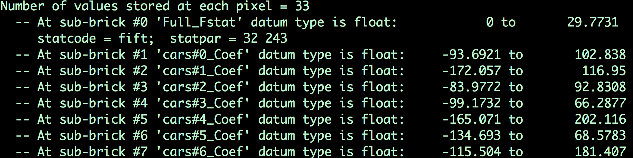
The contents of the file MVPA.BLOCK.nii. Remember that the first file is indexed as 0; in other words, the first sub-brik in this dataset is “#0 ‘Full_FStat’”, the first sub-brik for the Cars condition is sub-brik #1, which is labeled ‘cars#0_Coef’, and so on.
We will then extract the sub-briks from each class in the output of 3dDeconvolve, ``MVPA.BLOCK.nii`, using a for-loop. For example, to extract the sub-briks for the Car condition, we can use this line of code:
for a in $(seq 1 8); do 3dTcat -prefix cars.$a.nii MVPA.BLOCK.nii[${a}]; done
Which will create 8 files, cars.1.nii, cars.2.nii, all the way until cars.8.nii. (The seq command creates a string of numbers between the two arguments that are provided; in this case, 1, 2, 3, 4, 5, 6, 7, and 8.) We will use this same command to extract the corresponding sub-briks for the Faces, Houses, and Shoes conditions:
for a in $(seq 9 16); do (( b=`expr $a - 8` )); 3dTcat -prefix faces.$b.nii MVPA.BLOCK.nii[${a}]; done
for a in $(seq 17 24); do (( b=`expr $a - 16` )); 3dTcat -prefix houses.$b.nii MVPA.BLOCK.nii[${a}]; done
for a in $(seq 25 32); do (( b=`expr $a - 24` )); 3dTcat -prefix shoes.$b.nii MVPA.BLOCK.nii[${a}]; done
In this case, we include another piece of code, expr. Since we want to label each sub-brik we extract as corresponding to the first through the eighth of that condition, we subtract from the sub-brik number that is specified in the seq command. For example, the first sub-brik of the Faces condition is the ninth one in the MVPA.BLOCK.nii file; by subtracting 8 from 9, we label the first sub-brik as faces.1.nii, and so on for all of the sub-briks in that condition.
When you have finished running the code, you should see something like this:
01_Extract_sub-brik_output.png
Creating the Training Set
Now that we have the sub-briks, we will create a training set for the classifier. The classifier will then have some experience of what the typical beta map looks like for each of the conditions in our experiment, and will be able to make an educated guess about what condition an unlabeled beta map belongs to.
In order to avoid any ordering confounds, we will select at random beta maps from each condition. This can be done with a random number generator, such as the one in Excel; but for now, we will use the same beta maps that are listed on the Brown website. For example, we will select beta maps 3 through 8 for the Cars condition, leaving beta maps 1 and 2 for the training set:
3dTcat -prefix cars.train.nii cars.3.nii cars.4.nii cars.5.nii cars.6.nii cars.7.nii cars.8.nii
This will create a new dataset, ``cars.train.nii`, which contains beta maps 3 through 8. We will do a similar procedure for the other conditions, selecting different sets of beta maps:
3dTcat -prefix faces.train.nii faces.2.nii faces.8.nii faces.1.nii faces.7.nii faces.4.nii faces.5.nii
3dTcat -prefix houses.train.nii houses.5.nii houses.3.nii houses.4.nii houses.8.nii houses.6.nii houses.7.nii
3dTcat -prefix shoes.train.nii shoes.8.nii shoes.7.nii shoes.4.nii shoes.3.nii shoes.6.nii shoes.2.nii
We will then concatenate all of those training datasets into a single dataset called trainBlock.nii:
3dTcat -prefix trainBlock.nii cars.train.nii faces.train.nii houses.train.nii shoes.train.nii
In another file that was downloaded with the dataset, trainLabels.1D, we find a string of numbers:
1
1
1
1
1
1
2
2
2
2
2
2
3
3
3
3
3
3
4
4
4
4
4
4
Since there are 4 classes, we label each of the volumes in our training dataset trainBlock.nii with a number; in this case, 1’s for Cars, 2’s for Faces, 3’s for Houses, and 4’s for Shoes. The numbers are arbitrary - you can label them however you want, as long as the numbers within a category are consistent. You will need to remember these numbers when running the classifier on the testing data, which will return a number for its best guess as to the category for each condition.
Creating the Testing Set
With each training set containing 6 beta maps, the testing set will therefore contain the remaining 2 beta maps for each condition. These are the beta maps that the classifier will use to make a guess as to which condition they belong to:
3dTcat -prefix cars.test.nii cars.1.nii cars.2.nii
3dTcat -prefix faces.test.nii faces.3.nii faces.6.nii
3dTcat -prefix houses.test.nii houses.2.nii houses.1.nii
3dTcat -prefix shoes.test.nii shoes.5.nii shoes.1.nii
We then combine them into a single testing dataset, called testBlock.nii:
3dTcat -prefix testBlock.nii cars.test.nii faces.test.nii houses.test.nii shoes.test.nii
Creating the Mask
Just as with ROI analyses for fMRI data, we will want to restrict our analyses to a mask indicating which voxels to include for our analysis. Since we are doing a visual recognition task, we will want to restrict our analyses to the visual and temporal lobes of the brain; and, further, to the grey matter voxels of those lobes.
This mask has already been generated for you, in the file final.mask.nii. An axial view shows the voxels that will be used for our classification analysis:
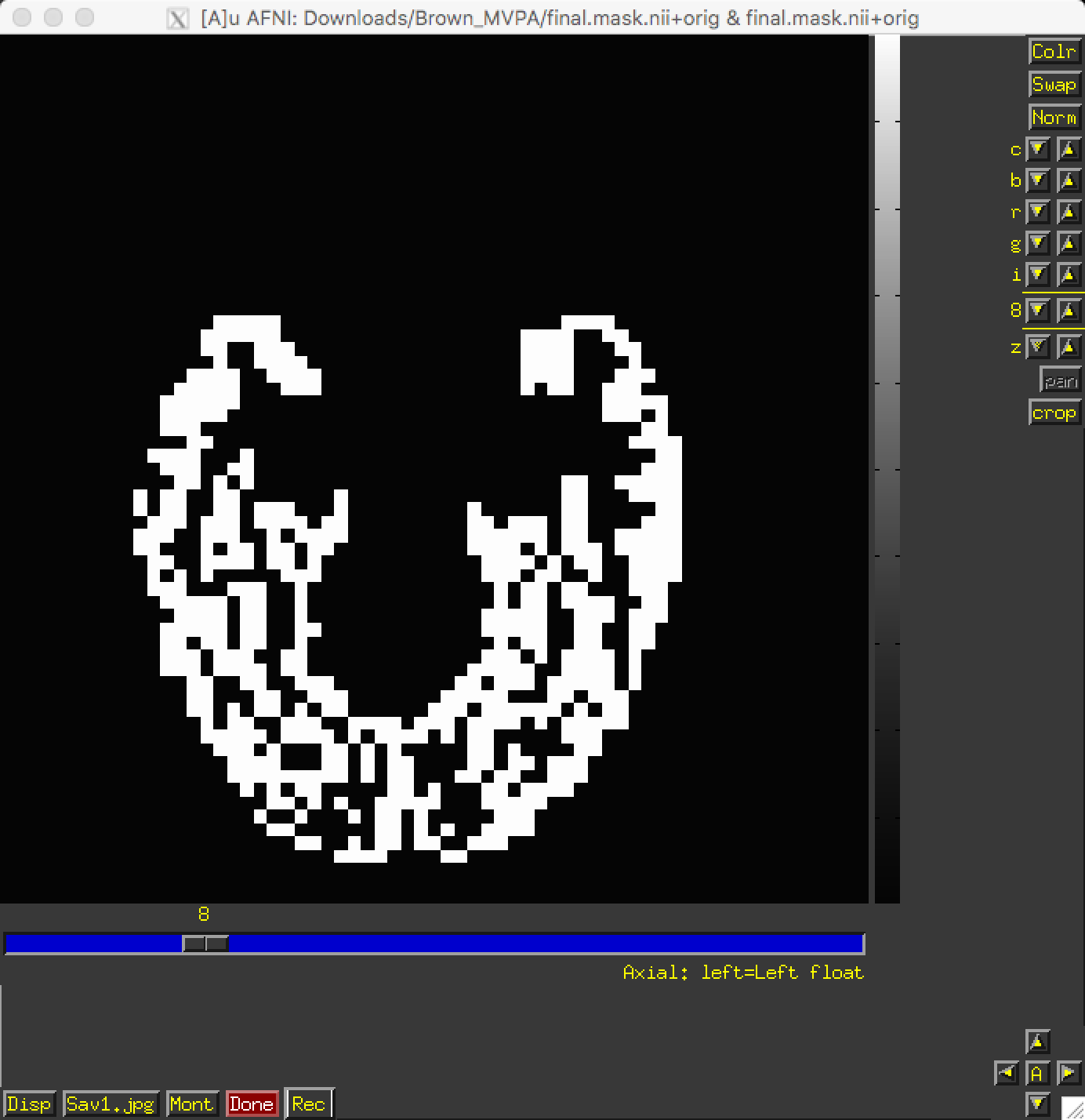
If the mask had not already been generated for you, other options would be to either 1) Create a spherical ROI based on the results of another study examining a similar region; 2) create a mask using regions defined by an atlas; or 3) Process the anatomical image through FreeSurfer and use the parcellations generated by recon-all. The choice is up to you.
Training and Testing the Classifier
Now that we have testing data for the classifier, we will show each beta map to it, along with the labels indicating which condition that beta belongs to - analogous to showing a person pictures of several different males and females to get a sense of what each category looks like. To do this, we will be using a support vector machine that attempts to draw a hyperplane between the pattern of voxels that best classifies each category.
To train the model, we provide the training dataset, the training labels, and the mask for our analysis; these are indicated by the options -trainvol, -trainlabels, and -mask, respectively. To output the model generated by the support vector machine, we will use the -model option:
3dsvm -trainvol trainBlock.nii \
-trainlabels trainLabels.1D \
-model trainSet.model.nii \
-mask final.mask.nii
We will then input this into 3dsvm again, using the testBlock.nii file as our testing volume:
3dsvm -testvol testBlock.nii \
-model trainSet.model.nii \
-classout \
-predictions exemplar
This command will use the training set generated in the previous command to predict which volume in the testing block belongs to which category. For example, we know that the first two volumes belong to the Cars category; since we labeled them as 1’s, the classifier - if it is accurate - should also classify them as 1’s. We then compare the classifier’s predictions to the actual labels in order to compute its accuracy. The -classout option will label each prediction as an integer, and -predictions will prepend a string to each set of predictions (in this case, “exemplar”).
Since we have 4 categories, the classifier generates a separate file for each combination: 1 vs. 2, 2 vs. 3, 2 vs. 4, and so on. If we look within the file exemplar_1_2.1D, we find the following:
1
1
2
2
1
1
1
2
In which the training block attempts to judge whether each volume in the training set belongs to category 1 or category 2; that is, whether it belongs to Cars or Faces. The first two volumes, which we know are the beta maps for the Cars category, have been correctly identified, although a few other beta maps have been identified as Cars although they are not.
You can look at the other combinations at your leisure. The most important file for our purposes, however, is exemplar_overall_DAG.1D. This file contains predictions for every combination of category that we used in our training dataset, and the output may look something like this:
1
3
2
2
3
3
1
4
As we saw before, the first two volumes are Cars, the second two are Faces, the third pair are Houses, and the last two are Shoes. Note that both Faces and Houses have been classified correctly, whereas Cars and Shoes are less accurately classified. If we were doing a group analysis, we would run this same classification for each subject and then add up the accuracies for each category. If there is a significantly higher classification accuracy for one category or group of categories compared to other categories, and the classification accuracy is greater than chance - in this case, greater than 1 in 4, or 25% - we can conclude that the voxels in our mask are able to reliably represent one category as opposed to another.
Why This Mask?
You may be wondering why we chose the voxels that we did - specifically, the ones located in the temporal and occipital lobes. These voxels were not chosen at random, but rather were chosen based on many studies that have shown that these voxels show reliable patterns of activation in response to faces. One of the classic studies of this phenomenon was conducted by Haxby et al., 2001; and it happens that we can download the data from that study and analyze it the same way. We will learn how to do that in the following chapters, in order to both consolidate what you’ve learned about MVPA, extend it to a group analysis, and replicate the results of a famous experiment.
Video
For a video demonstration of how to use 3dsvm, click here.