Machine Learning Tutorial #9: Representational Similarity Analysis

---

Overview

Representational Similarity Analysis (RSA)

Downloading the Data

The dataset for this analysis can be found here, on The Decoding Toolbox’s website. This folder contains the fully preprocessed and analyzed data for a single subject, with betas generated for each trial of each condition. After you have downloaded the dataset, move it to your Desktop directory, and look inside:

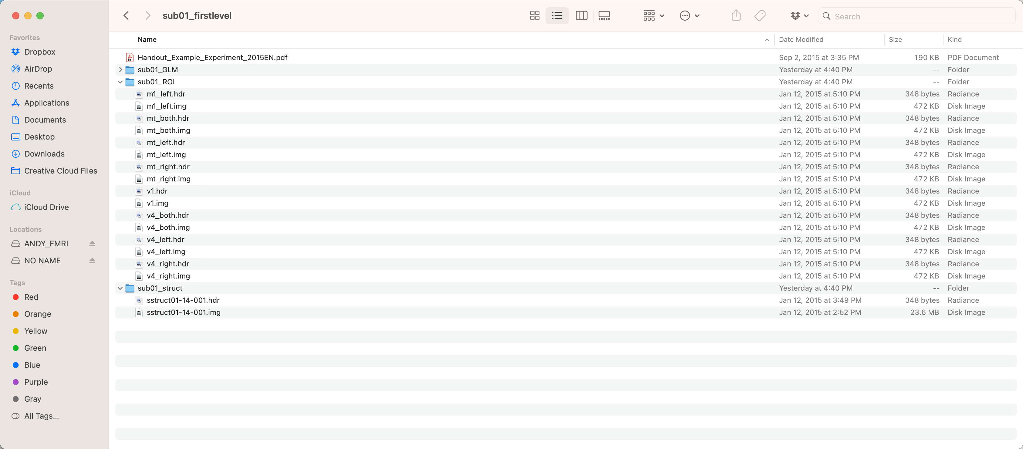
The folder sub01_GLM contains the betas estimated from the GLM; the folder sub01_ROI contains different ROIs that can be used for the classifications analysis, such as the left primary motor cortex and primary visual cortex; and sub01_struct contains the anatomical image. For this tutorial, we will be using the data in the GLM and ROI folders.

In this experiment, subjects were given instructions to respond to either the color of the stimuli, or the direction of the stimuli. After seeing either red or green dots move up or down, the subjects then responded with a left or right button press, mapped on to either the direction or the color of the stimuli.

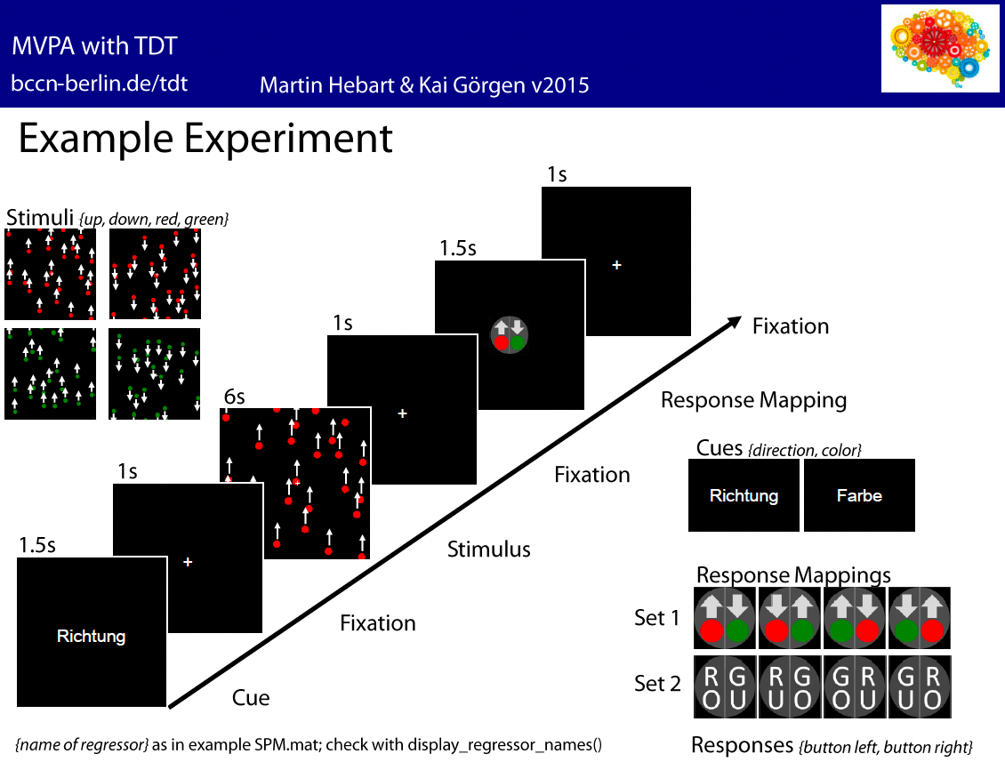
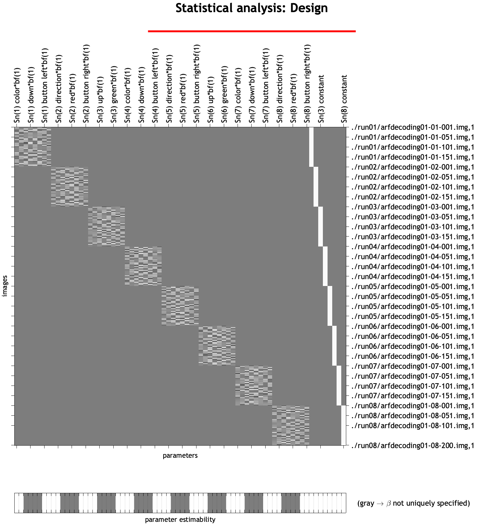
As a result, there were eight regressors entered into the model, in the following order (regressor name is in parentheses to the right of each one, as returned by the command display_regressor_names run in the directory sub01_GLM):

1. Instruction cue to respond to the color of the stimulus (color);

2. Instruction cue to respond to the direction of the stimulus (direction);

3. Stimuli moving in the “up” direction after the direction cue (up);

4. Stimuli moving in the “down” direction after the direction cue (down);

5. Red stimuli after the color cue (red);

6. Green stimuli after the color cue (green);

7. Left button presses (button left);

8. Right button presses (button right).

There are also constant, or baseline, regressors included at the end of each run to model the intercept, which we will ignore for our similarity analysis.

These can be verified in SPM by opening SPM12, clicking Review, and selecting the SPM.mat file in the sub01_GLM directory.

Creating the Script

The Decoding Toolbox has a template RSA script lcoated within tdt_3.999F/decoding_toolbox/templates; if your path already points to this folder, you can navigate to the folder sub01_firstlevel, and then type open decoding_template_similarity.m. Save a copy of it to the sub01_firstlevel folder, and call it RSA_SampleScript.m. Open this new file in your Matlab terminal by typing RSA_SampleScript.m, and close the original template script.

First, change the cfg.analysis on line 14 to from searchlight to ROI, since we will be using ROIs for our similarity analysis. The code on lines 17 and 20 specify where to write the results and where the betas are located, respectively; change them to cfg.results.dir = ``[pwd '/sub01_Results']; and beta_loc = [pwd '/sub01_GLM'];. Lastly, if we are interested in RSA in the left motor cortex, for example, we would change line 27 to be cfg.files.mask = [pwd '/sub01_ROI/m1_left.img'];.

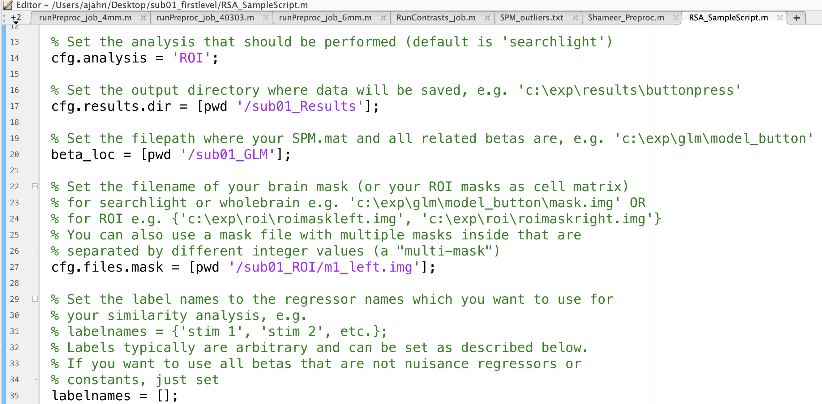
For now, leave the rest of the defaults as they are, noting on line 45 that the classification parameter output is set to pearson, i.e., correlation values. We will experiment with different options later, which can be found in the file pattern_similarity.m.

Note

If you want to save disk space and overwrite the results each time you run the script, add the line cfg.results.overwrite = 1; anywhere in your script before the last line (i.e., results = decoding(cfg)) I recommend doing this for the remainder of the tutorial.

Running the Script and Viewing the Output

You can now run the script by typing RSA_SampleScript. After a few seconds, you should see a new variable in your workspace called results. Within this structure is a field called other, which in turn has a sub-field called output. You can display all of the data in this matrix - in other words, all of the correlation values calculated for each condition - by typing reuslts.other.output{1}.

However, the output is quite large, and it is probably easier to view and understand the output if we plot it as a correlation matrix. To do that, type:

figure; heatmap(results.other.output{1}, 'Colormap', jet)

This will generate a plot that looks like this:

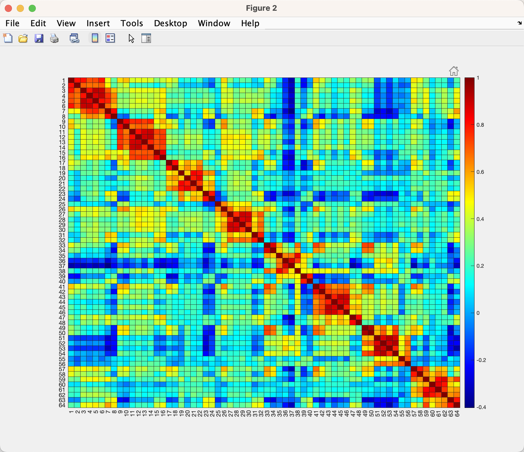
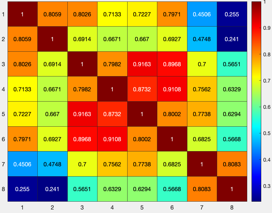
Note that there are 64 rows, and 64 columns, since there are 8 conditions and 8 runs. For example, the first column and second row (i.e., cell(1,2)) represents the correlation between the instructions for color and the instructions for direction, which in this case is 0.8059; you can verify this by hovering your cursor over that cell. (Also note that the matrix is symmetrical around the diagonal, and that the upper triangle is identical to the lower triangle.) You can see a clear pattern in the matrix, which appears to have eight separate 8x8 matrices running along the diagonal, representing within each run the correlation of the conditions with each another. There are correlations off the diagonal as well, which represent the correlation of a condition in one run with the condition in another run; for example, cell (1,9) represents the correlation between the instructions for color for run 1 with the instructions for color for run 2.

To simplify the matrix, let’s focus in on the first 8x8 matrix by typing:

figure; heatmap(results.other.output{1}(1:8,1:8), 'Colormap', jet)

Which will return a figure like this:

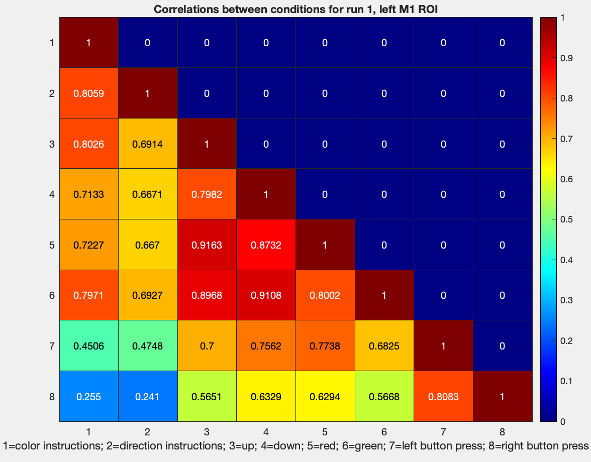
And if you want just the lower diagonal, you can type:

figure; heatmap(tril(results.other.output{1}(1:8,1:8)), 'Colormap', jet)

Along with a title to describe what we are looking at:

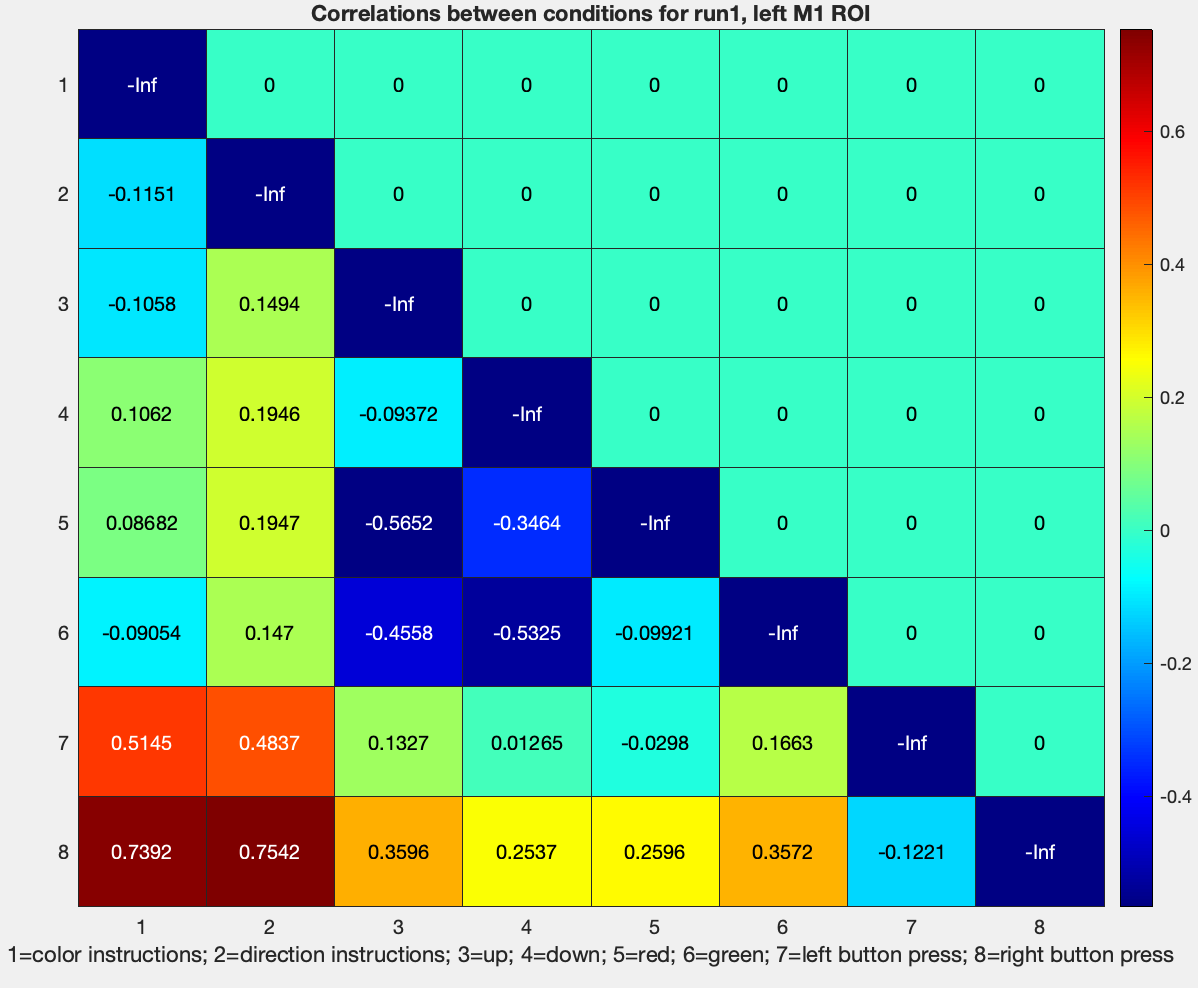
title('Correlations between conditions for run1, left M1 ROI')

And annotations along the x-axis:

xlabel('1=color instructions; 2=direction instructions; 3=up; 4=down; 5=red; 6=green; 7=left button press; 8=right button press')

The same procedure can be done for the other runs; for example, run 2 can be visualized with:

figure; heatmap(tril(results.other.output{1}(9:17,9:17)), 'Colormap', jet)

And so forth.

Creating Dissimilarity Matrices and Using Other Similarity Metrics

We have now generated similarity matrices. Remember, however, that we are interested in *dis*similarity matrices; a measure of how far apart two categories are, which can be measured from an absolute zero point. To that end, we will need to subtract these correlation values from 1, which can be done with a simple edit to a previous line of code:

figure; heatmap(tril(1-results.other.output{1}(1:8,1:8)), 'Colormap', jet); title('Correlations between conditions for run1, left M1 ROI'); ...
xlabel('1=color instructions; 2=direction instructions; 3=up; 4=down; 5=red; 6=green; 7=left button press; 8=right button press')

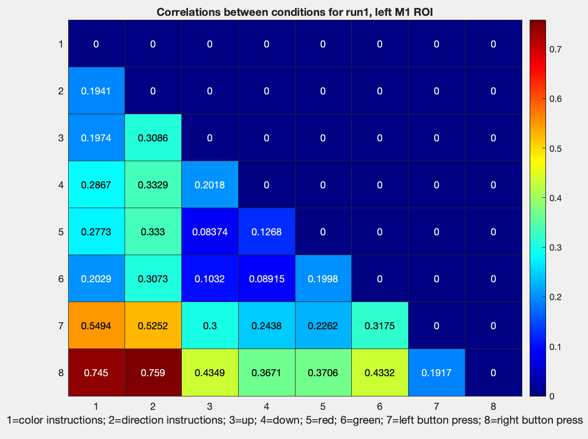
Note that the dissimilarity is relatively low for left and right button presses, which, given that we are looking at activity in the left motor cortex, should make sense. The highest dissimilarity is between left and right button presses, and the instruction cue for both color and direction.

If we wanted to run statistics on these values, it would probably be easier to use transformed r-to-z values, which are more normally distributed. In fact, there are many other similarity metrics you can use, which can be found in the documentation for the function pattern_similarity.m, located in The Decoding Toolbox libraries. The options have been reprinted below:

- 'gmatrix' or 'gma': X'*Y, commonly used in pattern component
    modeling, can be used to construct Euclidean distance
- 'cveuclidean2' or 'cve': will calculate the cross-validated
    version of the squared Euclidean distance between X and Y
- 'euclidean' or 'euc':  Euclidean distance
- 'Pearson', 'pea' or 'cor': Pearson correlation similarity
- 'zcorr' or 'zco': Fisher-z-transformed correlation similarity
- 'Kendall' or 'ken': Kendall's tau rank correlation similarity
- 'Spearman' or 'spe': Spearman's rho rank correlation similarity
- 'covariance' or 'cov': Sample covariance (divides by n-1)

We have used Pearson in the example above; let’s now change it to a z-transformed metric, by going back to our RSA_SampleScript.m and editing line 45:

cfg.decoding.train.classification.model_parameters = 'zcorr';

Rerun the script, and use the same code above to plot the z-transformed values, which should generate something like this:

These values can then be used to compute averages across runs, and then across subjects, and then between groups, as desired.

Comparing Dissimilarity across ROIs

So far, we have used the voxels within the left M1 for creating similarity matrices. To take this analysis a step further, we might be interested in comparing these dissimilarity matrices across ROIs. For example, how are the dissimilarity matrices different across the motor and visual cortices? We can use these differences to see how they provide evidence for or against certain computational models.

Continuing with this example, let’s add the visual cortex ROI to our analysis. We will edit line 27 of the RSA_SampleScript.m file to read:

cfg.files.mask = {[pwd '/sub01_ROI/m1_left.img'], [pwd '/sub01_ROI/v1.img']};

Keep all the other parts of the script the same, and run it from the command line by typing RSA_SampleScript. You will now have two sub-fields in the output field of the results structure; you can plot the Fisher-to-z transformed scores for the V1 ROI by typing:

figure; heatmap(tril(1-results.other.output{2}(1:8,1:8)), 'Colormap', jet); ...
title('Correlations between conditions for run1, V1 ROI'); ...
xlabel('1=color instructions; 2=direction instructions; 3=up; 4=down; 5=red; 6=green; 7=left button press; 8=right button press')

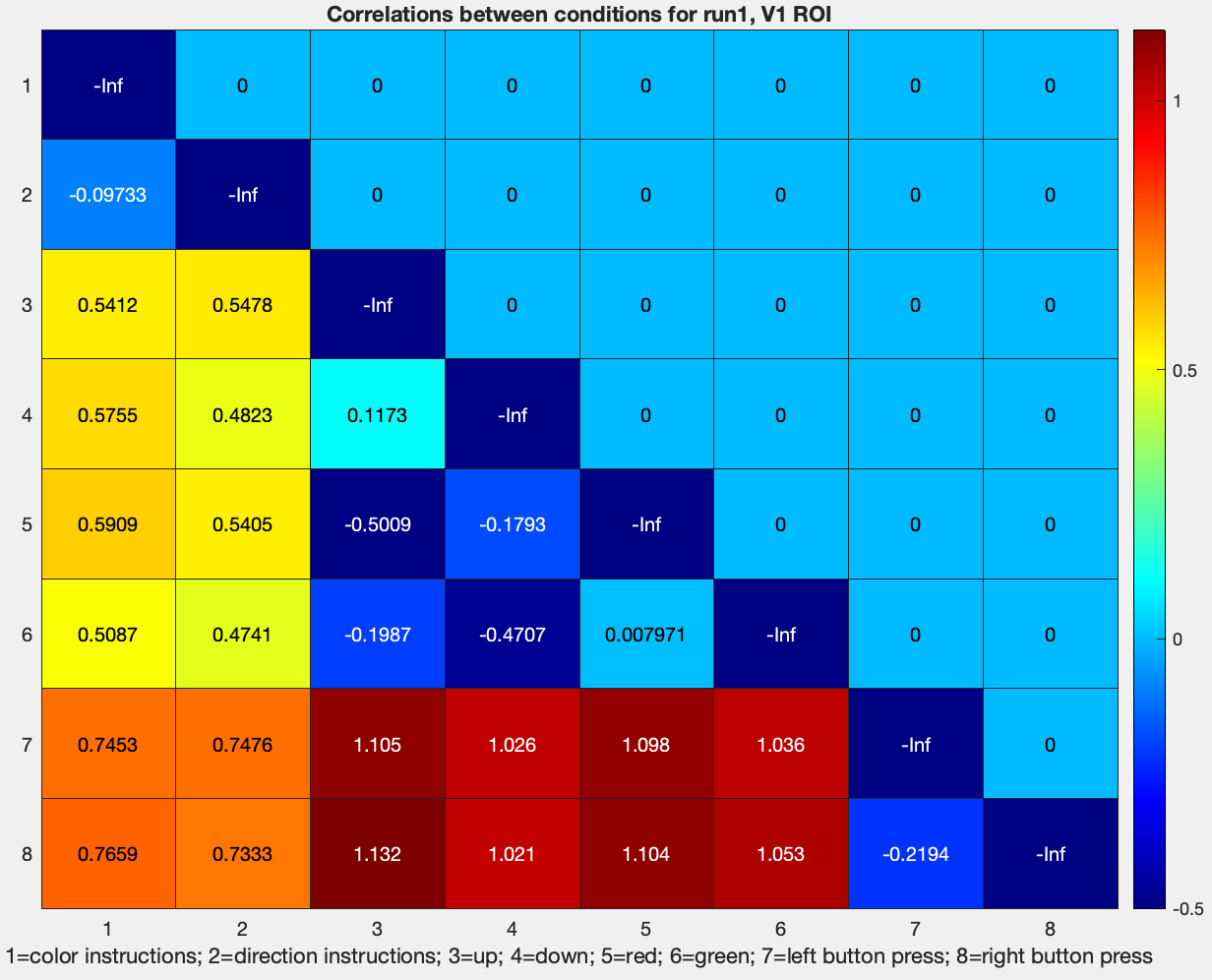
Note how the dissimilarity z-values between the conditions Red, Green, Up, and Down, are roughly similar to what they were in the motor cortex ROI. However, the dissimilarity of the Instruction cues with the other conditions, and of the button presses with the other conditions, are much higher. This could be because motor activity is represented very differently in the visual cortex than in the motor cortex, and because reading instructions elicits a different pattern of visual activity than simply viewing colored objects move up or down. How to interpret these differences is up to you.

Averaging Across Runs

Note

The following section should be equivalent to changing line 54 of RSA_SampleScript.m to cfg.results.output = 'other_average';; however, as of this time, it seems to give identical output to the code above.

To prepare the data for a group-level analysis, we will first need to average the similarity metrics across runs. In this case, since each run is an 8x8 matrix, we can extract the values with the following code:

ColorInstructions_ColorInstructions = mean(diag(1-results.other.output{1}(1:8:end,1:8:end)))
ColorInstructions_DirectionInstructions = mean(diag(1-results.other.output{1}(2:8:end,1:8:end)))
ColorInstructions_Up = mean(diag(1-results.other.output{1}(3:8:end,1:8:end)))
ColorInstructions_Down = mean(diag(1-results.other.output{1}(4:8:end,1:8:end)))
ColorInstructions_Red = mean(diag(1-results.other.output{1}(5:8:end,1:8:end)))
ColorInstructions_Green = mean(diag(1-results.other.output{1}(6:8:end,1:8:end)))
ColorInstructions_LeftButtonPress = mean(diag(1-results.other.output{1}(7:8:end,1:8:end)))
ColorInstructions_RightButtonPress = mean(diag(1-results.other.output{1}(8:8:end,1:8:end)))

DirectionInstructions_ColorInstructions = mean(diag(1-results.other.output{1}(1:8:end,2:8:end)))
DirectionInstructions_DirectionInstructions = mean(diag(1-results.other.output{1}(2:8:end,2:8:end)))
DirectionInstructions_Up = mean(diag(1-results.other.output{1}(3:8:end,2:8:end)))
DirectionInstructions_Down = mean(diag(1-results.other.output{1}(4:8:end,2:8:end)))
DirectionInstructions_Red = mean(diag(1-results.other.output{1}(5:8:end,2:8:end)))
DirectionInstructions_Green = mean(diag(1-results.other.output{1}(6:8:end,2:8:end)))
DirectionInstructions_LeftButtonPress = mean(diag(1-results.other.output{1}(7:8:end,2:8:end)))
DirectionInstructions_RightButtonPress = mean(diag(1-results.other.output{1}(8:8:end,2:8:end)))

And so on, for every other combination of conditions. These can then be concatenated together, and visualized as an 8x8 matrix.

Exercises

1. When you compute a dissimilarity matrix by subtracting the correlation values from 1, you may see that some values are greater than 1. Why is this? What does this mean about the similarity of that condition to another condition?

2. Run the same RSA analysis, this time with v4_both.img. (Remember that you can run multiple ROI analyses by using brace notation, e.g., cfg.files.mask = {[pwd ‘/sub01_ROI/m1_left.img’], [pwd ‘/sub01_ROI/v1.img’], [pwd ‘/sub01_ROI/v4_both.img’]}.) How are the similarity matrices different? How are they similar? Why do you see these differences or similarities? Show the output from each dissimilarity matrix for each analysis.