fMRIPrep Tutorial #5: Running the 1st-level Analysis
Overview
In the AFNI tutorial on 1st-level analysis, we learned how to create a General Linear Model to estimate the BOLD response to each condition in our experiment. We will be doing the same thing here, extracting the relevant motion confound regressors from the .tsv file generated by fMRIPrep.
Examining the Confound Regressors File
fMRIPrep creates a confound file for each run; for example, the confound regressor file for run 1 is called sub-08_task-flanker_run-1_desc-confounds_regressors.tsv. If you open this file in a spreadsheet program such as Excel, you will see the following:
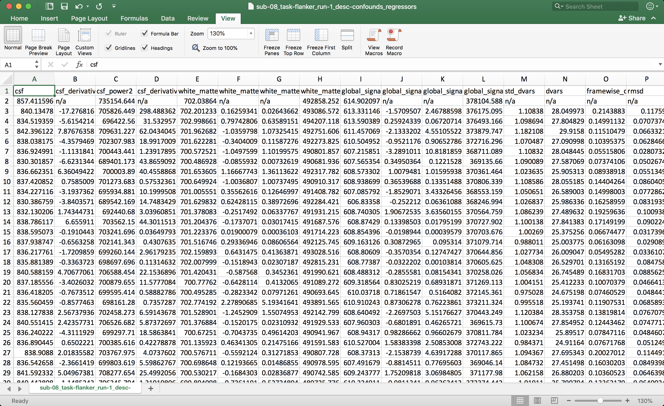
You can see that the file contains many confounds, and you probably won’t use all of them. If we wanted to replicate our AFNI analysis as closely as possible, however, we will need to find the motion regressors in the x-, y-, and z-directions. The translation regressors can be found in columns EU, EY, and FC; while the rotation regressors can be found in columns FG, FK, and FO. Note that the location of these regressors may change from subject to subject, depending on how many components are extracted during ICA analysis of the different tissues.
There are several other regressors that you can include, such as global signal, framewise displacement, and different component time-series. Which ones to include are up to you; in any case, remember to use these regressors with AFNI’s stim_files options, which will not convolve the time-series with a basis function, such as the HRF.
Converting the Timings
Before we can run the 1st-level analysis, we will need to convert the timing files; the steps for doing this can be found here. The paragraph to follow is pasted below:
To format the timing files, download this script. (You can download it by clicking on the
Rawbutton, then right-clicking in the newly-opened window and selecting “Save As”.) We won’t go into detail about how it works, but all you need to do is place it in the experimental folder containing the subjects (i.e., theFlankerdirectory), and typebash make_Timings.sh. This will create timing files for each run for each subject and store them in each subject’s correspondingfuncdirectory. To check the output, typecat sub-08/func/incongruent.1D. You should see numbers similar to the ones in the figure above.
When you have generated the timings, navigate to the fmriprep output directory for sub-08 in the derivatives folder, and type the following:
mkdir stimuli
cp ../../../../sub-08/func/*.1D stimuli
This will place the timing files within the stimuli directory.
Modifying the Confound Regressor Files
Before we can insert our confound regressors into the General Linear Model, we will need to do a few steps in Unix to format them correctly. AFNI expects a separate regressor file for each run, with later runs containing a string of zeros equal to the number of volumes in the previous run. For example, if we have two runs with 146 volumes each, the second regressor file should have 146 zeros before the first confound regressor.
First, we will create a backup of the second confound regressor file:
cp sub-01_task-flanker_run-2_desc-confounds_regressors.tsv run-2_confounds_regressors_BACKUP.tsv
And then create a for-loop to extract the translation and rotation parameters for the x-, y-, and z-directions. The awk and sed commands will print the numbers in each of those columns, and then put them in files that either contain just the header, or everything except the header:
for reg in trans_x trans_y trans_z rot_x rot_y rot_z; do
  for run in 1 2; do
    awk -v col=$reg 'NR==1{for(i=1;i<=NF;i++){if($i==col){c=i;break}} print $c} NR>1{print $c}' sub-08_task-flanker_run-${run}_desc-confounds_regressors.tsv > ${reg}_run${run}_all_tmp.txt;
    sed '1d' ${reg}_run${run}_all_tmp.txt > ${reg}_run${run}_noHead_tmp.txt
    sed '1!d' ${reg}_run${run}_all_tmp.txt > ${reg}_run${run}_Head_tmp.txt
  done
done
We will then create a string of zeros equal to the number of volumes in the previous run:
NT=`3dinfo -nt r1_scale.nii`
if [ -f zeros_tmp.txt ]; then rm zeros_tmp.txt; fi
for ((i=0; i<$NT; i++)); do echo 0 >> zeros_tmp.txt; done
Concatenating the two files using cat will generate a file that can now be read by AFNI:
for reg in trans_x trans_y trans_z rot_x rot_y rot_z; do
  for run in 1 2; do
    if [ $run -eq 1 ]; then
      cat ${reg}_run${run}_noHead_tmp.txt > ${reg}_run${run}.txt
    else
      cat zeros_tmp.txt ${reg}_run${run}_noHead_tmp.txt > ${reg}_run${run}.txt
    fi
  done
done
rm *tmp*
Creating the 3dDecon File
We now have all of the ingredients we need to run the 1st-level analysis: timing files, preprocessed functional data, and a mask. To run this through 3dDeconvolve, click on this link, click on the Raw button, and then right-click and select “Save As”. Save the file into the folder derivatives/fmriprep/sub-08/func, and then navigate to that directory with a terminal and type the following:
tcsh doDecon.sh sub-08
This will run the 1st-level analysis for sub-08. When it is finished, you can open the stats.tlrc file in the AFNI viewer and overlay it on the template “MNI152_2009_template.nii.gz”. If you threshold the image at p=0.001, change the color scale to red/blue, check the Pos? box, and clusterize it at n=40, you should see something like the figure below:
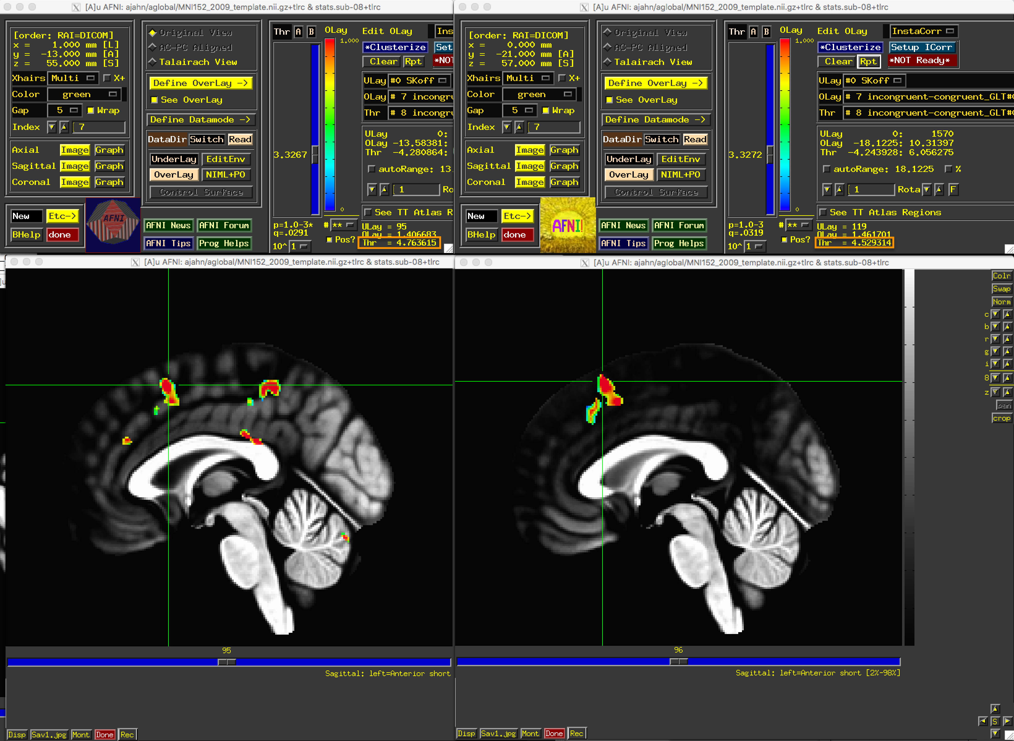
The fMRIPrep results are shown on the left; the original results using the AFNI pipeline are shown on the right. Note that the basic pattern of activity is the same, and that the peak t-statistic in the mPFC is slightly higher in the fMRIPrep version.
Next Steps
Now that we have successfully analyzed a single subject, we now move on to a group-level analysis. To learn more about how to do that, click the Next button.
Video
A video demonstration of performing a first-level analysis can be found here.