Chapter 6: Running the First-Level Analysis

---

uber_subject.py Revisited

Previously, we used the command uber_subject.py to set up the preprocessing script for a single subject. You may recall that we removed one of the processing blocks, called “regress”, because we were not focusing on regression at the time. Now, however, we will add the regress block back into our uber_subject.py script, and combine both preprocessing and 1st-level analysis into a single script.

Let’s create a new script for the same subject, sub-08. First, remove the preprocessed directory by navigating to the sub-08 directory and typing rm -r subject_results. From the directory containing all of your subjects, type uber_subject.py from the command line. This time, in the “analysis initialization” section, we will leave all of the blocks as they are (although since the data in this example dataset are already slice-time corrected, you could remove the “tshift” block without affecting the results, as discussed in an earlier chapter).

Fill in the anatomical and functional images as you did for preprocessing, and keep make the same changes to the “extra align options” and “extra tlrc options”. The sections of the GUI we will focus on in this chapter are: stimulus timing files; symbolic GLTs; and extra regress options.

Note

If uber_subject.py isn’t working, you can download the output script here.

Stimulus Timing Files

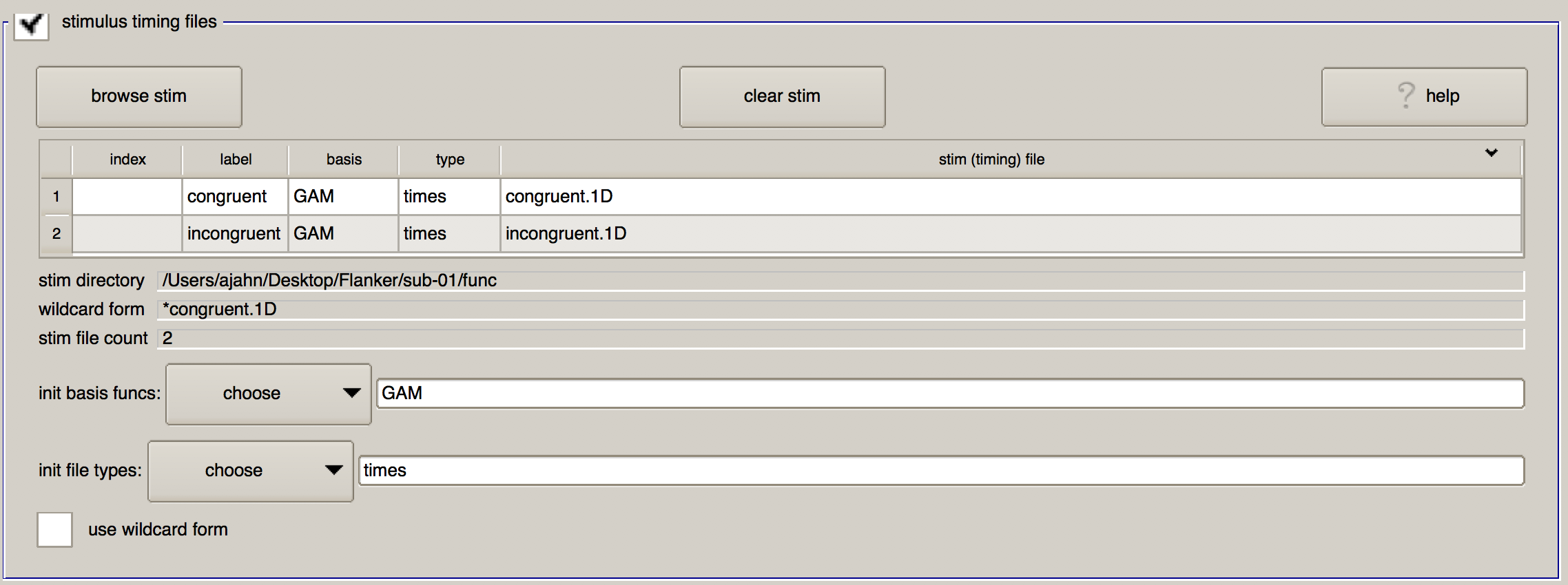
Having created the timing files in the previous chapter, click on the “browse stim” button and select the files congruent.1D and incongruent.1D located in sub-01/func. (You can select multiple files by holding down the command key and clicking on individual files.)

When you click “OK”, you will see a table populated with the timing files you selected. In addition to showing the name of the timing file you selected, there are three other columns named “label”, “basis”, and “type”. “Label” is how the timing file will be reference in the command that does the model fitting (i.e., 3dDeconvolve), whereas “basis” and “type” specify which basis function to apply to the timing files.

The default basis function of GAM specifies that the onset times should be convolved with the canonical HRF discussed in a previous chapter. This basis function requires that only one parameter be estimated - namely, the height of the HRF, which roughly corresponds to the amount of neural activity in response to that condition. Other basis functions that you can apply are the BLOCK function (i.e., the boxcar regressor that was discussed in the chapter on the HRF), a TENT function which estimates the activity at specified time-points after the onset of the condition, and SPMG2, which includes a temporal derivative.

The field below, “init file types”, allows you to specify the type of convolution you wish to use. The default of times means to convolve all of the time-points specified in the timing file and generate a parameter estimate for the HRF that on average fits all of the occurrences the best; IM, on the other hand, will estimate a separate beta weight for each trial (which can be used, e.g., for more advanced analyses such as beta-series analysis). The AM1 and AM2 options are used for parametric modulation analyses (which are beyond the scope of the present tutorial), and files indicates that no convolution should be applied - which is useful for nuisance regressors such as motion.

When you have finished loading the files, this part of the GUI should look as follows:

Symbolic GLTs

The next section, “Symbolic GLTs”, allows you to specify general linear tests that will be calculated after the beta weights above are estimated for the conditions above. The notation is a little strange, and it is probably easiest to click on the “init with examples” button to show example syntax for setting up the tests. When you do, you will see two contrasts: C-I, and mean.CI.

Let’s look at the first contrast: This uses contrast weights to specify how the contrast between different conditions will be calculated, and it prepends the contrast weights to the labels specified in the “stimulus timing files” section. No sign implies a contrast weight of +1, while a negative sign implies a contrast weight of -1. Therefore, the line congruent -incongruent means to weight the parameter estimate for the Congruent condition with +1, and to weight the parameter estimate for the Incongruent condition with -1, and then to take the difference between the two. Using a different computation, the second contrast takes the average of the two conditions by multiplying both by 0.5.

Note

As a general rule, contrast weights that compute a difference between conditions should sum to 0, and contrast weights that take an average across conditions should sum to 1.

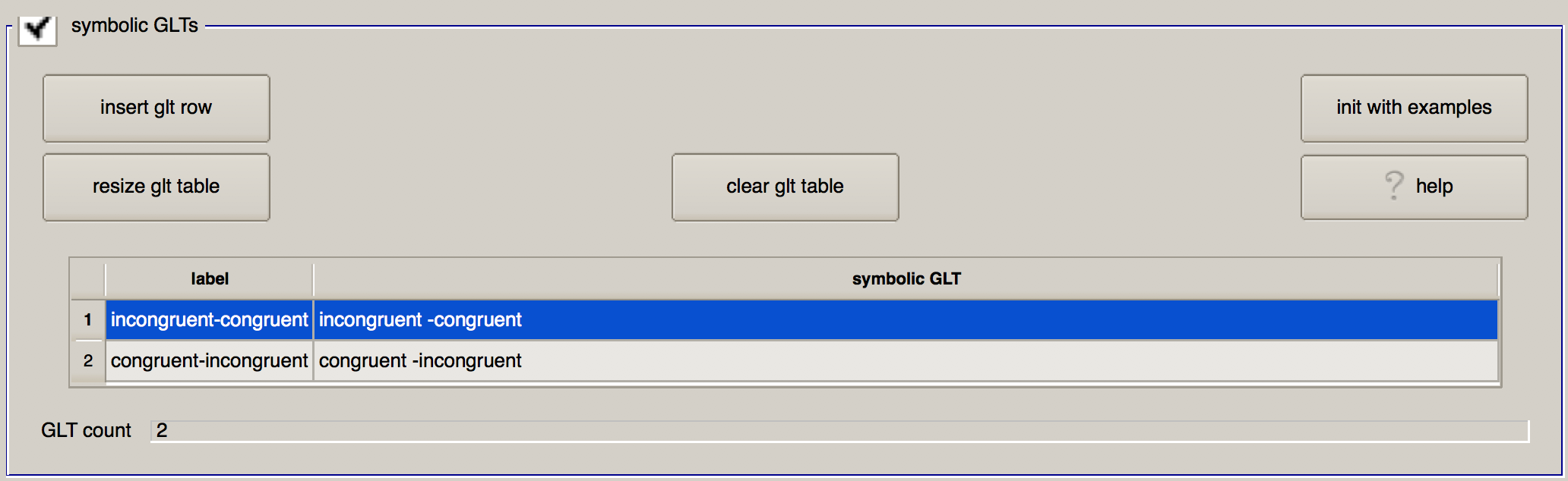
Let’s modify this table to practice the GLT syntax, and to set up the contrasts that we want. In the first row, change the “label” column to incongruent-congruent, and in the “symbolic GLT” column, type incongruent -congruent. Likewise, in the second row specify a contrast of congruent-incongruent. When you have finished, the section should look like this:

Extra Regress Options

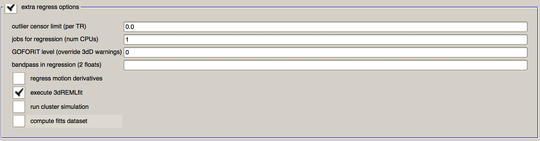
Lastly, we will indicate any preferences we have for the 3dDeconvolve command. The first field, “outlier censor limit”, will remove any TRs from the analysis that have a censored outlier fraction greater than the amount specified in the field to the right. (These outliers are detected by 3dToutcount, which flags any voxels in a TR that have signal intensity greater than 3 standard deviations from the other voxels in brain mask.) If this is left at 0.0, then no TRs will be censored based on the output from 3dToutcount. We will leave this as is for now, since volumes with high amounts of motion will be censored.

The next field, “jobs for regression (num CPUs)”, specifies how many processors to use for the regression analysis. Since this step can be computationally demanding, use the maximum number of CPUs that you can spare. In this case, I will set it to ``8`.

“GOFORIT level (override 3dD warnings)” will ignore any warnings about the design matrix detected by 3dDeconvolve. In general, you should not use GOFORIT unless you are positive that the matrix error is negligible. In general you will want 3dDeconvolve to throw a warning and stop running when it detects an abnormally high level of collinearity among two or more regressors.

The “bandpass in regression” field is usually for resting-state analyses, in order to remove both low and high frequency fluctuations. For task data, however, low-pass filtering (i.e., removing high frequency signal) risks removing actual signal related to the task. Leave this blank.

There are four checkboxes in addition. “Regress motion derivatives” will model higher-order derivatives of the motion regressors, which can capture more complex head movements. This is useful for populations that tend to move a lot, such as children or certain clinical subjects; and as long as you have a long time-series of data (e.g., more than 200 TRs in a run), you probably won’t run out of degrees of freedom for estimating these extra parameters. For this tutorial I will leave it unchecked, but you are free to do whatever you want.

I also leave the “run cluster simulation” box unchecked, as this computes whether a cluster is statistically significant in real time as you change the thresholding slider. Since I generally don’t perform inference on single subjects - we will do inference later at a group level - I omit this option. I do, however, check the “execute REMLfit” option, as this will create a separate statistical dataset that better accounts for temporal autocorrelation than the traditional 3dDeconvolve approach. Later on, we can use the output from 3dREMLfit to use information about the variability of the subject’s parameter estimates in order to create more precise group-level inference maps.

When you are done, this section should look like this:

Now, click the top three icons in succcession (the sheet of paper, the magnifying glass, and the green “Go” button) to run both the preprocessing and the regression. In total, it should take about 5-10 minutes.

The Ideal Time-Series and the GLM

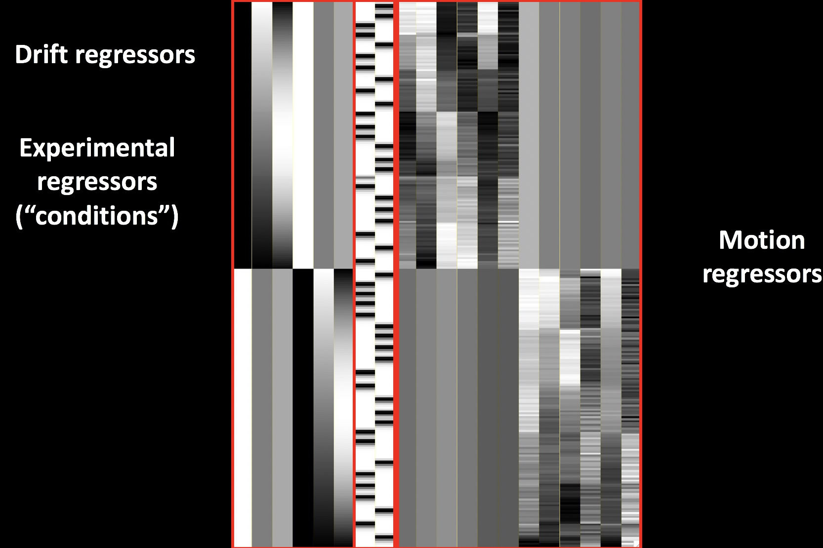
While you’re waiting for the analysis to finish, let’s take a look at how the model we just created relates to the GLM. Remember that each voxel has a BOLD time-series (our outcome measure), which we represent with Y. We also have our two regressors, which we will represent with x1 and x2. These regressors constitute our design matrix, which we represent with a large X.

So far, all of these variables are known - Y is measured from the data, and x1 and x2 are made by convolving the HRF and the timing onsets. Since matrix algebra is used to set up the design matrix and estimate the beta weights, the orientations are turned ninety degrees: Normally we think of the time axis as going from left to right, but instead it is depicted as going from top to bottom. In other words, the onset of the run begins at the top of the timecourse.

The next part of the GLM equation is the beta weights, which we represent with B1 and B2. These represent our estimate of the amount the HRF needs to be scaled for each regressor to best match the original data in Y - hence the name “beta weights”. The last term in this equation is E, which represents the residuals, or the difference between our ideal time series model and the data after estimating the beta weights. If the model is a good fit, the residuals will decrease, and one or more of the beta weights are more likely to be statistically significant.

Examining the Output

When the script finishes, navigate into the folder sub-08/subject_results/group.Flanker/subj.sub08/sub08.results. In addition to the preprocessed blocks you saw previously, you will also see statistical datasets: The one labeled stats.sub_08+tlrc has been analyzed using the traditional 3dDeconvolve approach; the dataset stats.sub_08_REML+tlrc has accounted for temporal autocorrelation.

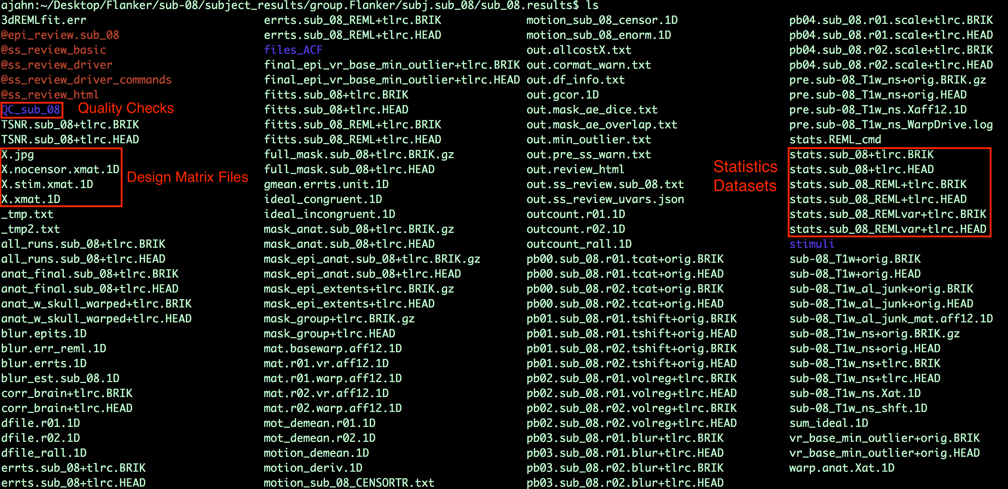
You will also see a few files beginning with an “X”, such as X.xmat.1D. These represent different parts of the design matrix. For example, you can view the design matrix by typing aiv X.jpg:

For a different view, looking at all of the regressors in separate rows, type 1dplot -sepscl X.xmat.1D:

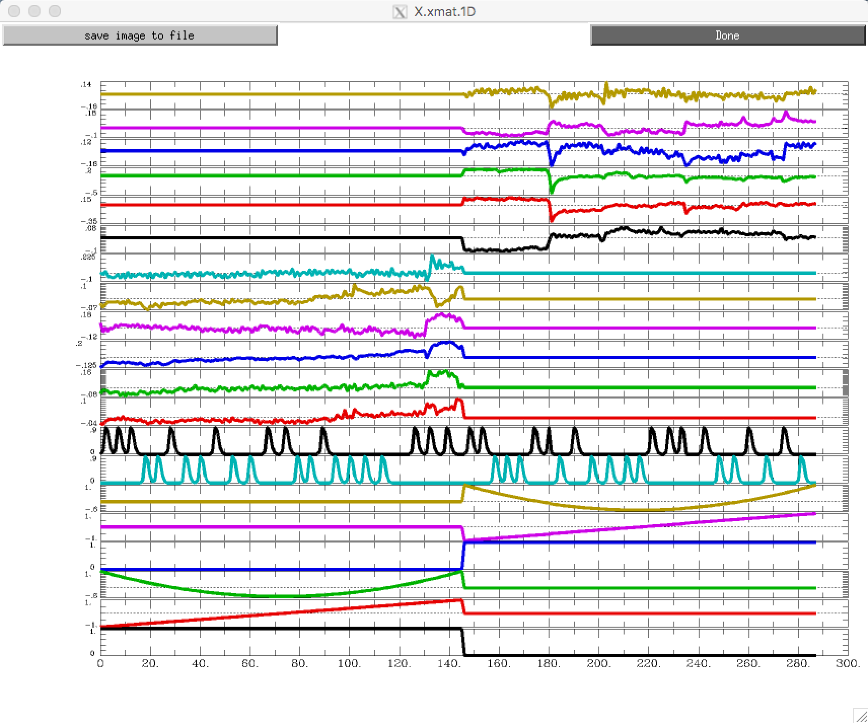
If you rotate this figure by 90 degrees, you will see that it is a different representation of the same design matrix above.

Note

Make sure the design matrix looks reasonable. Are the lower-frequency drifts modeled as you would expect them to be? Do the onsets for the trials in each condition match up with the timing files that you created in the last chapter?

Viewing the Statistics Files

We are now ready to look at the contrast maps of our data. Type afni to open up the GUI, and select anat_file.sub_08 as the Underlay. (You can also use the MNI152 template if you’ve copied it into your current directory, or if you have placed it in the aglobal directory.) For the Overlay, select stats.sub_08. You should see something like this:

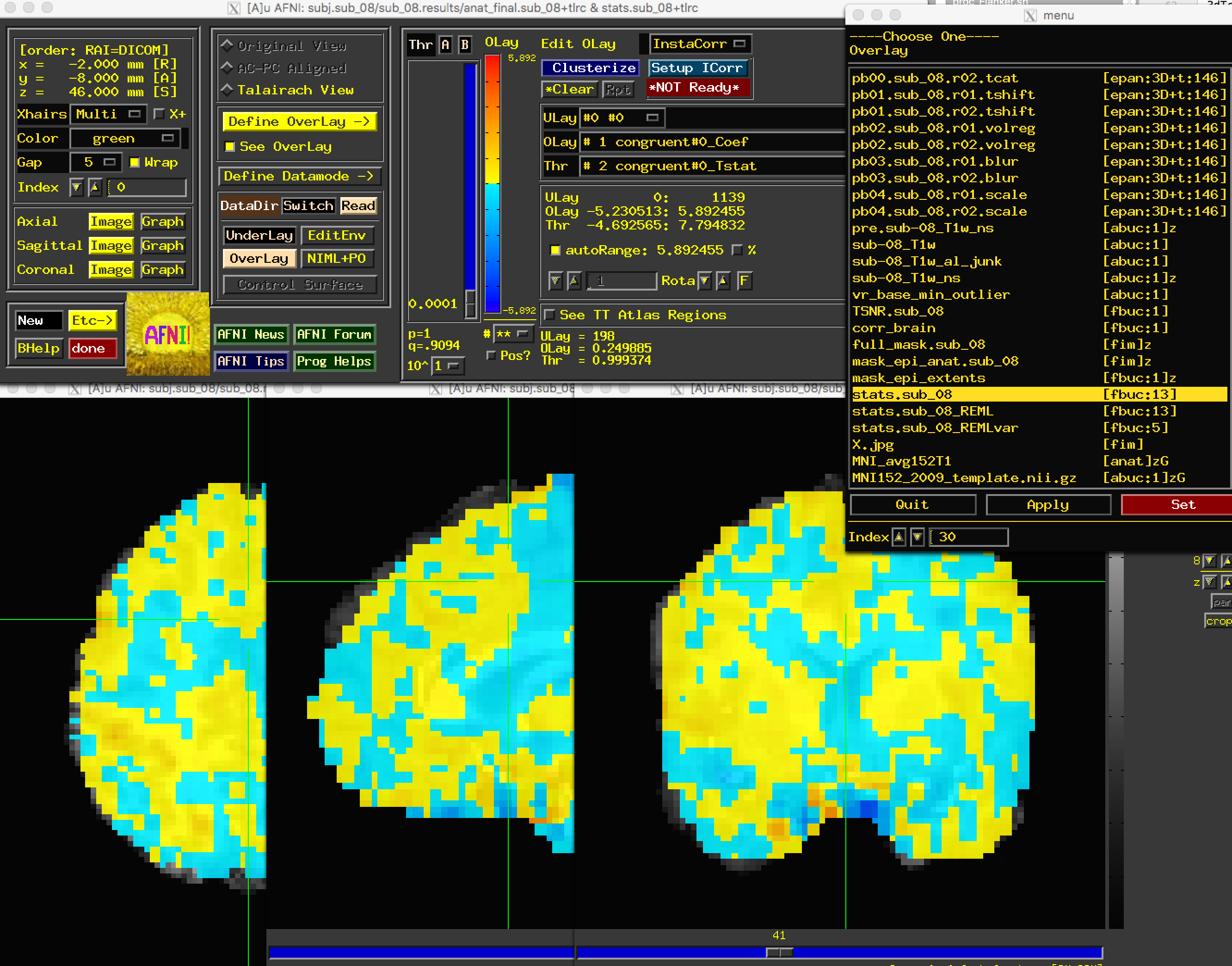
This may look overwhelming at first; but although the AFNI viewer can seem to have too many options, once you become more familiar with them you will be able to customize how you view your results. If this is your first time viewing statistics in AFNI, the most noticeable features of the “Define Overlay” panel will appear to be the slider bar (allowing you to threshold the images to only see values above a certain number), and the “ULay”, “OLay”, and “Thr” menus, corresponding to the Underlay, Overlay, and Threshold sub-briks.

Let’s begin with the slider bar. If you move it up and down, you will see voxels either disappear or re-appear. That is because we are thresholding, or removing, voxels that fall below the Threshold number to the left of the bar. This number will be based on the sub-brik that is selected in the “Thr” menu; in this case, the sub-brik that was selected for us when we opened the viewer was volume #2, the T-statistic map of the beta weights for the Congruent condition. As you move the slider to a value of, say, 1.9753, you will also notice that the number below the slider bar, p=, changes as well, to a value of 0.493. This represents the uncorrected p-value threshold for the currently selected Threshold map; in other words, any colored voxels pass an individual p-value threshold of 0.493.

Note

If you want to set a specific uncorrected p-value threshold, right-click on the p= text, select “set p-threshold”, and type the threshold you want (e.g., 0.001).

We haven’t corrected for multiple comparisons yet, so we can’t say whether any one of the individual voxels is statistically significant. However, viewing the data at an uncorrected p-value threshold can give you a general idea of the spatial layout of the statistics, and indicate whether the results are trending in the direction that you would predict, or if there appears to be something wrong. For example, highly correlated regressors would have very large parameter estimates and correspondingly high variability. You should also make sure that the activation, for a relatively high uncorrected p-value threshold (e.g., p=0.01 or higher), generally falls within the gray matter. If you find large numbers of “active” voxels within the ventricles, for example, it may indicate a problem with the data quality.

Now, change the OLay sub-brik to incongruent-congruent#0_Coef and the Thr sub-brik to incongruent-congruent#0_Tstat, and set the uncorrected p-value threshold to 0.05. Click around the brain, observing where the statistics are positive and where they are negative. Where do you notice significant “clusters” of activated voxels? Are they where you would expect them to be?

Later on, you will learn about a multiple correction technique called cluster correction. This method looks for clusters composed of voxels that pass a given uncorrected threshold, and then determines whether the cluster is significant or not. In this chapter we won’t go into how to calculate how large the cluster needs to be, but for now click the “*Clusterize” button and change the number of voxels to 45. As a result, you will only see those clusters that are composed of 45 or more voxels that each pass an uncorrected p-value threshold of 0.05. You can click on the “Rpt” button to see a report of each cluster that passes this threshold, which lists the voxel size, the location of the peak voxel of the cluster, and options to move the crosshairs to the cluster and make it flash. All of these operations are summarized in the video link below.

Exercises

1. In the lower right corner of the “Define Overlay” panel, you will see text that says OLay = and Thr =, and certain numbers on the right side of the equals sign. These indicate the value of the Overlay and Threshold datasets at the voxel where the crosshair is located; in other words, the parameter (or contrast) estimate, and the associated t-statistic. Select sub-brik #4 (incongruent#0_Coef) as an overlay, and write down the corresponding number that shows up in the OLay = field. Do the same thing for sub-brik #1 (congruent#0_Coef). Now select sub-brik #7 (incongruent-congruent_GLT#0_Coef), but before you do, think about what you would expect the value to be. Now select the sub-brik. Does it match what you predicted? Why or why not?

2. Do the same procedure in Exercise #1, looking at the contrasts of sub-briks #7 and #10. What do you notice about the value of the Overlay? Does this make sense given the contrast weights?

3. You can take the difference between beta weights by using an Image Calculator. Each of the major software packages has one; AFNI’s calculator is called 3dcalc. Take the difference between the Incongruent and Congruent betas for sub-08 by navigating to sub-08.results, and typing 3dcalc -a stats.sub-08+tlrc'[4]' -b stats.sub-08+tlrc'[1]' -expr 'a-b' -prefix Inc-Con+tlrc. The way to read this command is that it assigns the 4th sub-brik of the stats dataset to variable “a”, and the 1st-sub-brik of the stats dataset to variable “b”. We know that these correspond to the Incongruent and Congruent beta weights, respectively, and then we contrast them by typing the mathematical expression “a-b” in the -expr option. We then provide a prefix of our choice, in this case, “Inc-Con”. The resulting output should be identical to what you what you see in the results viewer when you use Inc-Con as an overlay. Now do the same procedure to create an output file called “Con-Inc”, which contrasts the 1st sub-brik with the 4th sub-brik.

4. Although the default color scheme and display are good enough for most purposes, you will probably want to change it to suit your own taste and aesthetics. For example, once you have thresholded your statistical overlay, click on the Define Datamode button in the AFNI GUI, click on Warp OLay on Demand, and select the Cu resampling method (for “Cubic” interpolation) for the OLay Resam mode. This will smooth the edges of the voxels that survive the threshold you used. Going back to the Define Overlay panel, right click on the color bar, and sample different color palettes to see which one you like best.

Next Steps

When you have finished running the preprocessing and first-level analyses, we will then need to run this for each subject in our study. To speed up the process, we will learn about scripting, to which we now turn.

Video

A video walkthrough of how to set up and review the first-level analysis can be found by clicking here.