Chapter #7: Denoising

---

Overview

One of the most important steps for cleaning up resting-state data is Denoising. Of course, removing noise is necessary for any imaging analysis; but as mentioned previously, resting-state data is particularly susceptible to artifacts such as linear drifts and motion effects.

To begin Denoising the data, click Done from the Setup tab. A new menu will appear, prompting you to select which resting-state analyses you want to do: Any combination of ROI-to-ROI, Seed-to-Voxel, and Voxel-to-Voxel. All three are selected by default; unless you only want to focus on a subset of these analyses, leave them as they are for now. Click Start to begin the Denoising step.

Note

You can change the default analyses by clicking on the “Options” button at the bottom of the Setup menu and checking or unchecking different analyses. You have control over other options as well, such as the resolution of the output data, what type of mask will be used, and whether to use parametric or non-parametric methods for determining the statistical significance of the results. You also have the option of generating additional output files, such as first-level seed-to-voxel r-maps. These can be useful if you want to use the connectivity maps for analyses outside of the CONN toolbox - such as The Brain Connectivity Toolbox.

The Denoising Tab

After a few minutes, you will have access to the Denoising tab. The window in the left upper corner shows the confound regressors that are used to account for different sources of noise, while the window on the right shows how much signal explained by each regressor. We will call these two general areas the the Denoising Settings area, and the Preview area.

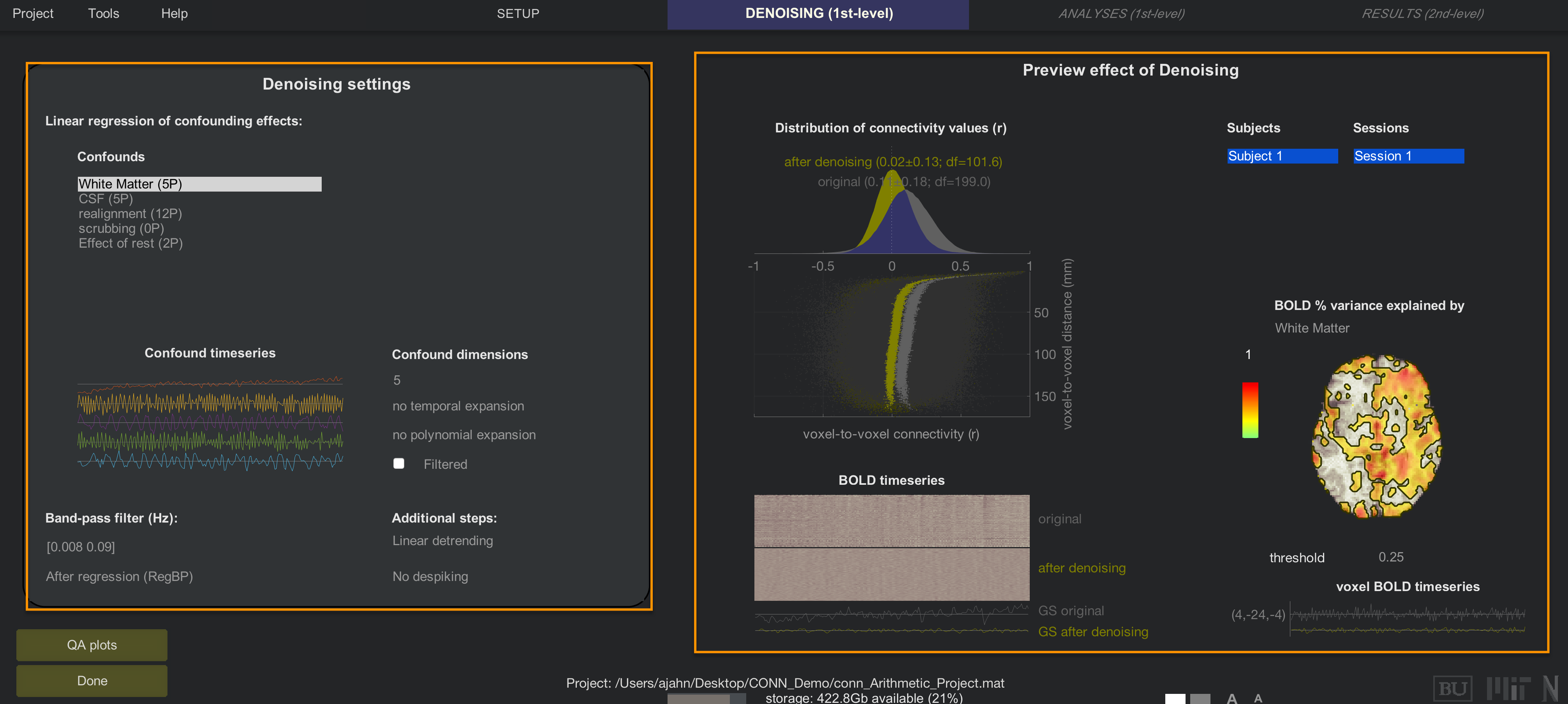
The area on the left displays a list of confound regressors that you can enter into your model, while the panel on the right shows the effect of including those regressors.

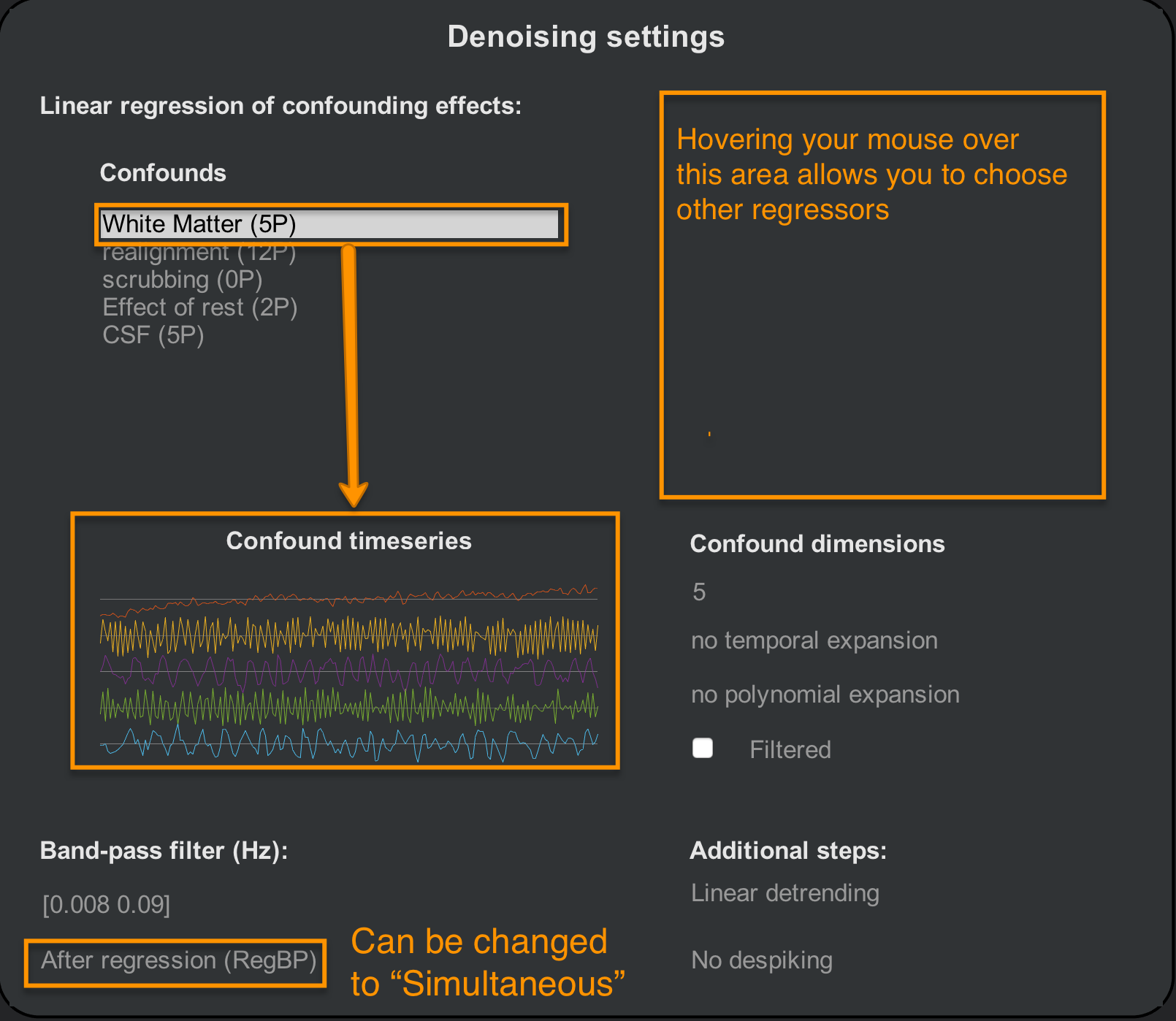
Denoising Settings

By default, CONN will include regressors derived from the tissue types you generated in the ROIs section of the Setup tab, and the 1st-level covariates of the Setup tab. CONN extracts five principal components from both the White Matter and CSF ROIs to best represent the signal profile in those regions. If you click on the string White Matter (5P), below you will see an illustration of each component’s time-series. In the “Confound dimensions” panel you can change the number of components; for example, try entering a value of 10, and see how the time-series panel changes.

Note

Although including more components can filter out more signal that is representative of white matter and cerebrospinal fluid, you quickly reach a point of diminishing returns. More regressors also means more degrees of freedom, which can reduce the statistical power of your model. For most experiments, the default of 5 components will be enough.

Within this panel, you can also choose to add higher-order temporal derivatives. If this is done at all, it is usually added to the motion regressors; 1st- and 2nd-order derivatives can capture more subtle movements that are not accounted for by the traditional translations and rotations. Polynomial expansion is a similar concept, adding either a quadratic or cubic exponent to the regressor, although this is not commonly done.

The Filtered checkbox specifies whether the regressor should be bandpass filtered before it is entered into the model. You can do this for individual regressors by highlighting the Confound regressor and checking the box, or by changing the After regression (RegBP) option to Simultaneous. In the Additional steps panel you can also choose to add higher-order detrending - for example, if you have a very long scan session and you think you may need to model more complex scanner drift - and Despiking. Despiking will artificially lower the signal of voxels that are abnormally high, and which are not accounted for by high motion. For most data, choosing to either Despike or not Despike will give similar results; however, for unusually noisy data, Despiking can be useful for removing artificially high signal.

Warning

Bandpass filtering the time-series data and then doing nuisance regression has been shown to re-introduce noise frequencies and components; see the Hallquist et al. (2014) paper for more details. The CONN toolbox doesn’t appear to have an option that will let you do this, but it is good to be aware of it in any case.

Note

If you want to remove either bound of the bandpass filter, enter Inf for that bound. For example, if you want to remove all of the lower frequencies below 0.008, but allow all higher frequencies, you would enter the vector [0.008 Inf].

Preview Denoising

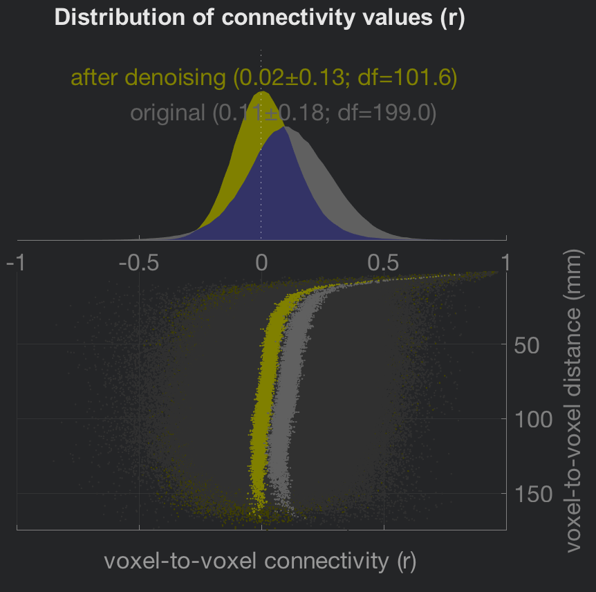
The right-side area of the Denoising tab will automatically update a figure showing how the regressors load onto the resting-state data. The distributions at the upper-left show the effect of your denoising regressors and parameters both before and after they are applied. In general, resting-state data is skewed to generate positive correlations, mostly as a result of the confound regressors such as motion. Note how the distribution of connectivity values is centered closer to zero after denoising is applied. The scatter plot below the distributions shows another view of the same principle: Data that is denoised shows a more uniform distribution in connectivity values as one tests for correlations at voxels farther away from the seed voxel.

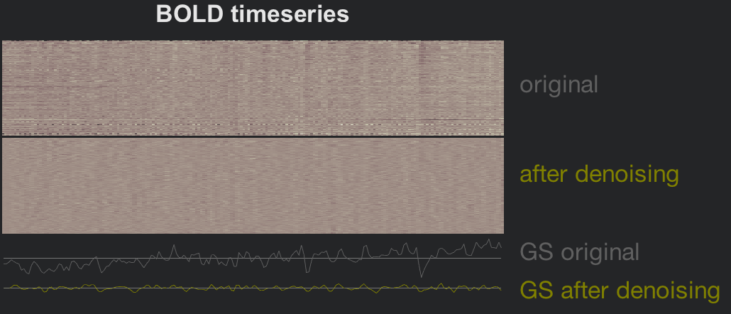
The figure in the lower-left side is a carpet plot which unravels each volume from a three-dimensional cube of voxels into a two-dimensional plot of squares. Each column represents an individual volume, and each row is an individual voxel in that volume. Denoising smooths out the rougher transitions between voxels that are probably caused by movement, scanner drift, and physiological noise; and the time-series plot of the global signal reflects this smoothing as well.

Lastly, the preview brain on the right-hand side shows the percent of variance in the BOLD signal explained by the currently highlighted confound regressor. The loading of the explained variance should correspond to the regressor that is highlighted. For example, can you guess which nuisance regressor this plot represents? What clues do you see? Try to guess what the figure would look like if one of the other confound regressors were selected.

Video

For a video overview of Denoising, click here.

Next Steps

For most datasets, the above figures should look similar - the distribution of connectivity values will be centered close to zero, and the BOLD timeseries will be smoothed out. If the data passes those checks, you are ready to begin estimating a general linear model using those regressors. To see how to do this, click the Next button.

Exercises

1. Enter a bandpass regressor of [0.008 Inf]. In your own words, describe what this filter will do. Is this in general better or worse than a low-pass filter? Why?

2. Experiment with highlighting different regressors in the Confounds window and checking the Filtered box, and observe what happens in the Preview window. Does this filtering (equivalent to the Simultaneous option in the After regression dropdown menu) seem to worsen or improve the nuisance regression? How would you make that judgment?

3. In the Denoising settings window, you add Gray Matter (1P) to the list of Confounds. Would this be considered Global Signal Regression? Why or why not? If not, what would you have to do for it to be true Global Signal Regression, and why? (For more information, see this post.)