Appendix D: Surface-Based Connectivity
Overview
The analyses you did in the previous chapters were done in what is called volumetric space; each image has individual voxels acquired with a specific length, width, and height, and the time-series is averaged across groups of voxels within each region. This works well for most purposes; however, functional connectivity can suffer from the same problems as task-based analysis during the preprocessing step of smoothing. As pointed out in a recent paper by Brodoehl et al. (2020), smoothing can average signal across functionally heterogeneous areas, which can be especially problematic for connectivity analyses. For example, the ridges of two nearby gyri can be a few millimeters away from each other when viewed from above, even though the actual distance from peak to peak - traveling along the ridge of the gyrus, like going down from one hill into a valley, and up the other hill - can be many times longer than that.
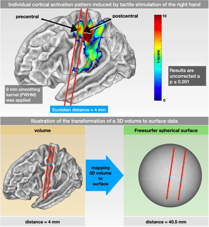
Figure 1 from Brodoehl et al. (2020). Note that the Euclidean distance (i.e., “as the bird flies”) between adjacent ridges of cortex can be as close as four millimeters. The actual distance from ridge to ridge, traveling through the valleys of the cortex, is ten times as long.
This distance is more accurately represented by reconstructing the image into surface space. Simply put, performing task-based and functional connectivity analyses on the surface allows the use of larger smoothing kernels without the signal contamination problems of smoothing in volumetric space. This can both increase power and reduce the chance of smoothing across regions or different tissue types. (More details about the differences between volumetric and surface-based analysis have been detailed in the SUMA module.) For the rest of the chapter, you will need to be familiar with FreeSurfer; the walkthrough can be found here. Once you have finished that tutorial and learned how to use the recon-all command, follow the steps below to modify your CONN project to analyze surface data.
Creating the Surface
For the remainder of this tutorial, we will use the first three subjects of the Arithmetic task on OpenNeuro.org, which can be found here. If you followed the steps in the previous chapters, you should have the entire dataset downloaded. Navigate to the folder Arithmetic, and type the following code:
for i in sub-01 sub-02 sub-03; do
  cd $i/anat;
  SUBJECTS_DIR=`pwd`;
  recon-all -s $i -i ${I}_T1w.nii -all;
  cd ../..;
done
This will run recon-all sequentially in each anat directory. Alternatively, if you have multiple processors on your computer, you could open three separate terminals and run recon-all in each of them; or, you could use the parallel command. The latter two options will complete recon-all more quickly by processing each subject in parallel. In any case, you should be able to process all three subjects in about a day.
Loading the Surface Data into CONN
When recon-all finishes, you will have a new directory within each subject’s anat folder. Each of these FreeSurfer directories will contain subfolders such as mri and surf, which you will need to import the surface data into CONN.
First, open a Matlab terminal and open the CONN toolbox. Create a new project called Arithmetic_Surface, which will open the Setup Tab. Enter 3 for the number of subjects, and change the TR to 3.56.
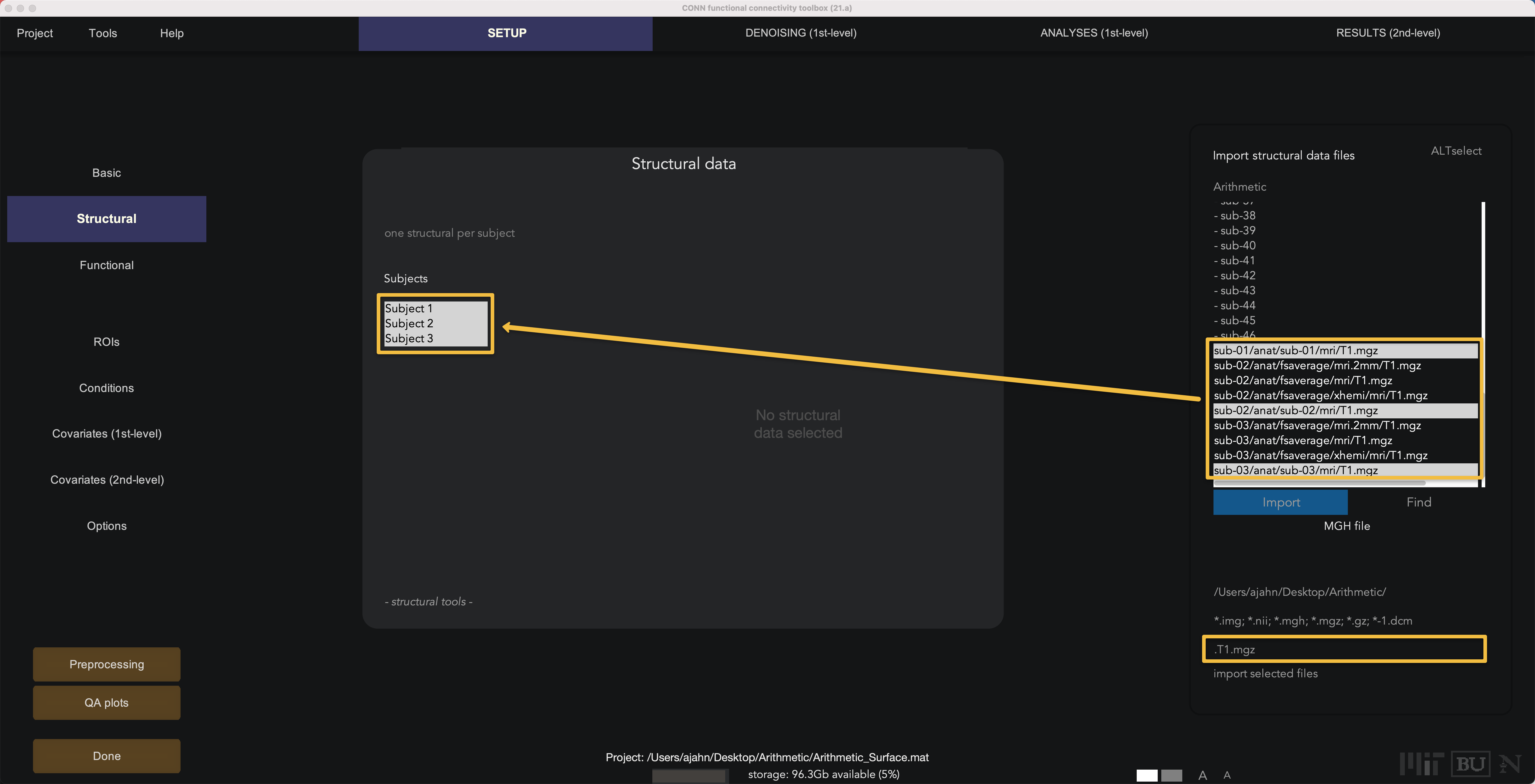
Next, click on the Structural button. Within the FreeSurfer output directories, there is a file called T1.mgz in the mri subfolder. In the Find field, type T1.mgz and then press the Find button; you should see a new list of files that contain the string T1.mgz. Shift and click to highlight all of the Subjects in the Structural data field, and then hold control and left-click to select the corresponding T1.mgz files for each subject, and click Import. This will automatically detect the surface reconstructed anatomical file, along with any segmentation files. If the aseg.mgz files are loaded, you can skip the segmentation step during preprocessing (discussed in more detail below).
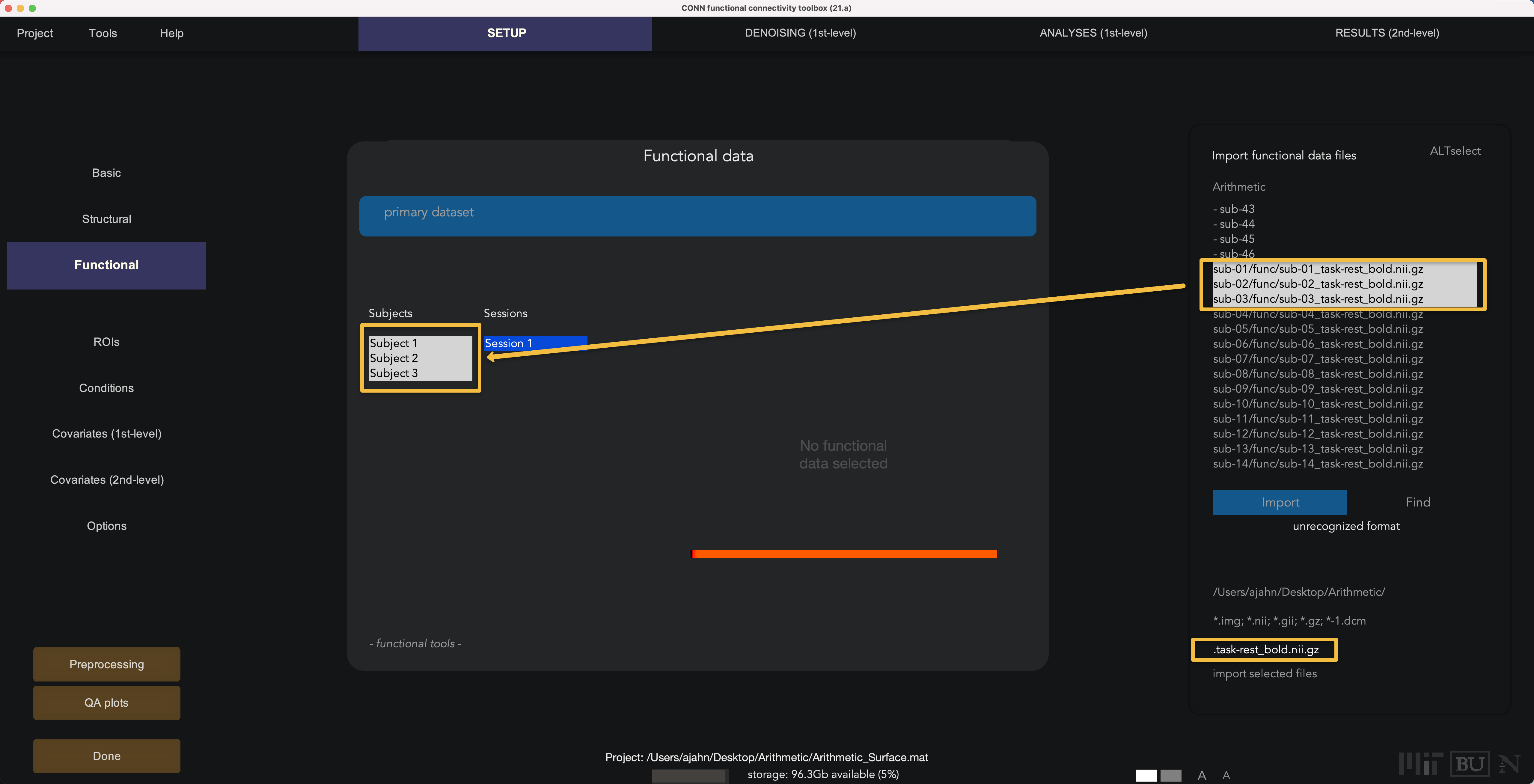
The functional data, by contrast, is still in volumetric space; during preprocessing, it will be resampled to surface space. Click on Functional. Similar to what we just did above, enter task-rest_bold.nii.gz in the Find field; highlight the three subjects in the Functional data window and then control and click to select their corresponding functional files.
Loading the FreeSurfer ROIs
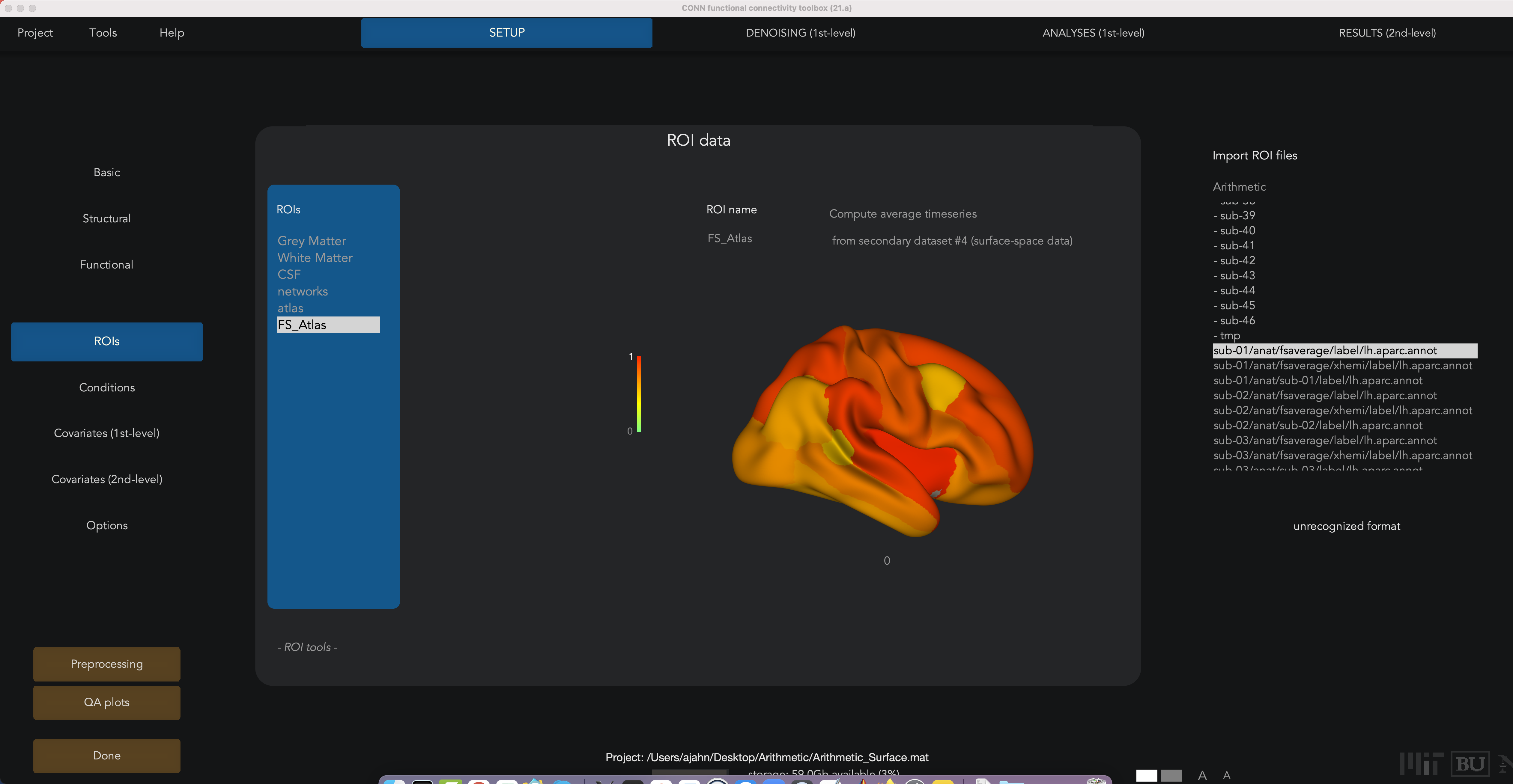
Even though the CONN toolbox doesn’t have a FreeSurfer atlas that comes with it, you can create it through the Setup tab. Click on the ROIs button, and then hover your cursor over the ROIs window and click the new button at the bottom of the window. Call the new ROI FS_Atlas, and in the “Find” field type lh.aparc.annot. (It doesn’t matter whether you use the left hemisphere or right hemisphere; the ROIs for both will be loaded automatically.) Select the file sub-01/anat/fsaverage/label/lh.aparc.annot, and then click Import. When it is finished importing, make sure the box Atlas File is checked at the bottom of the window.
Running the Preprocessing
Before you preprocess the images, first click Options and change the Analysis space (voxel-level) to Surface: same as template (Freesurfer fsaverage). This will carry out all of the first- and second-level analyses on the FreeSurfer fsaverage template, which is in MNI space. I would also uncheck the Voxel-to-Voxel button, to save time; you can perform this analysis later if you want.
Next, click the Preprocessing button, and select preprocessing pipeline for surface-based analyses (in subject-space). If you have the time and the processing power, you can choose the nonlinear coregistration option, which takes longer but generates a more accurate resampling of the volumetric data to surface space. In this example, I will remove slice-timing correction (since I don’t know how the slices were acquired in this experiment), and also segmentation, since the anatomical images were already segmented by FreeSurfer, and the segmentations were imported.
When the preprocessing finishes, go back to the ROIs section, and click on FS_Atlas. Under Compute average timeseries, select from secondary dataset #4 (surface-space data). This will use the averaged time-series from the resampled grey matter on the surface, instead of the volumetric data. When you have finished all of this, click the Done button to run the Setup pipeline.
Note
Once preprocessing has finished, you can see the functional connectivity maps on the individual subject surfaces by clicking on the Functional button. Similar to volumetric analysis, you will see the first volume on the left-hand side, and the last volume of the time-series on the right-hand side.
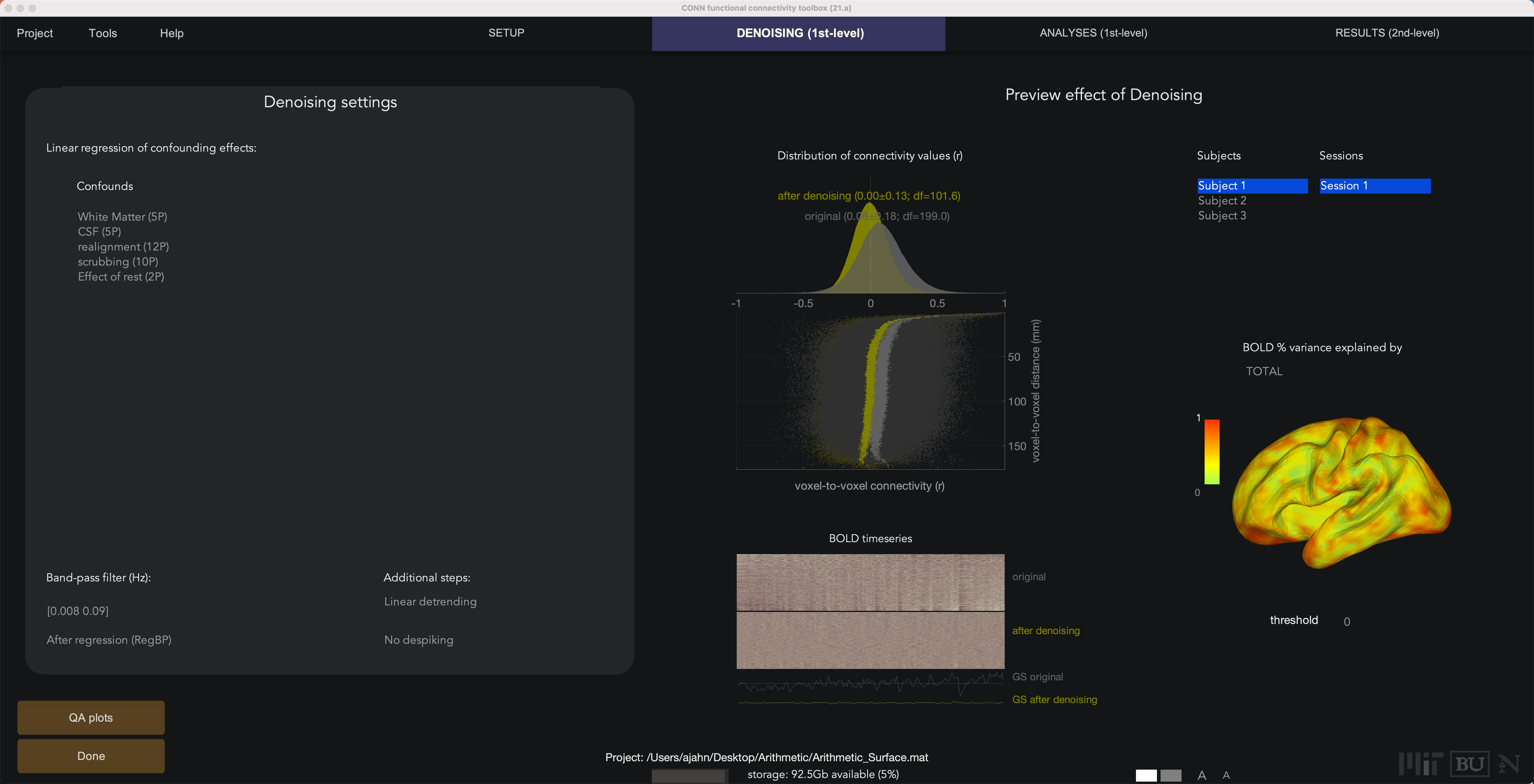
Denoising
The Denoising tab will be the same as was during the volumetric functional connectivity analysis, and the interpretation of the connectivity distributions and principal components correction is the same. The only difference is that you will see the BOLD variance projected onto a surface for each subject, instead of their volume.
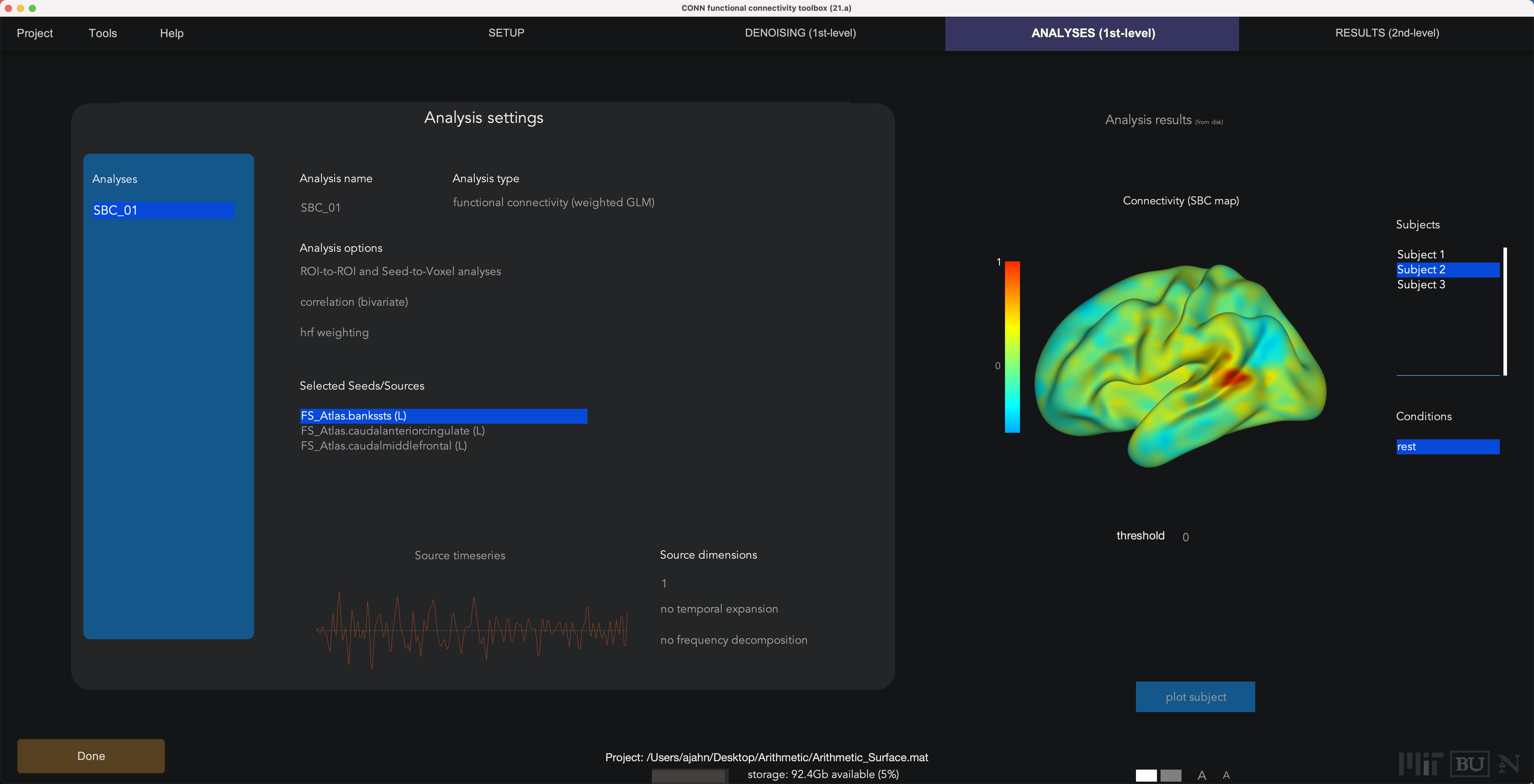
First-Level Analysis
The First-Level Analysis tab will also be very similar to a volumetric analysis, except that this time the results are projected onto a cortical surface. To save time, we will remove all of the Selected Seeds/Sources except for the first three ROIs listed in the FS_Atlas that we specified in the Setup tab: the FS_Atlas.bankssts (L), FS_Atlas.caudalanteriorcingulate (L), and FS_Atlas.caudalmiddlefrontal (L). Keep all the other defaults the same, then click the Done button; once it is finished, you can return to this tab and see connectivity maps for each ROI that was specified.
Second-Level Analysis
Once the first-level results are done, you can highlight any of the regions and click the compute results button. This will display a group-level result in the 2nd-level tab, and also generate a window with a glass brain and a corresponding table of significant clusters. If you click on the Surface Display button (the first one in the upper-left corner of the buttons under Display&Print, you can more accurately see the connectivity results displayed on the surface of the cortex.
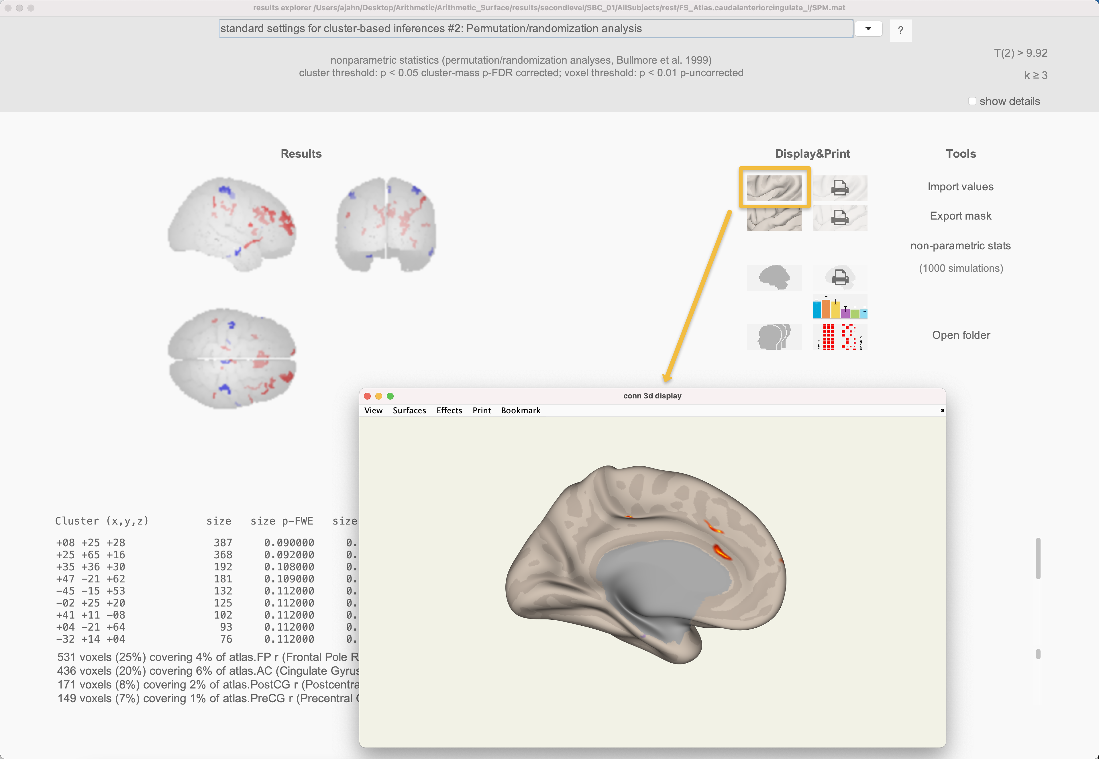
Note
As of the current version used in these tutorials (21.a), it does not appear that both subcortical and surface-based cortical parcellations can be combined in the same analysis; see this thread for more details.
Video
For a video demonstration of how to do a surface-based analysis in the CONN toolbox, click here.
Next Steps
All of the other options for volumetric-based analysis, including independent-samples tests, adding covariates, and ROI-to-ROI analyses, are the same in this case as well; the only difference being that the results are displayed on the surface. See the previous chapters for a walkthrough on how to run these other analyses.