Chapter #8: 1st-Level Analysis
Overview
The next step of our analysis is a 1st-level model. The regressors specified during the Denoising step, along with any condition regressors that were set in the Setup tab, are used to construct a model to best fit the data observed in each voxel. A correlation analysis is then computed, averaging across the signal in each of the ROIs and correlating it with other ROIs in the brain, along with generating correlation maps using each voxel as a seed.
To run the 1st-level model, click Done from the Denoising tab. A new menu will appear, similar to the one you saw before denoising: You have options for which type of resting-state analyses you want to do. Leave all of the boxes checked for now, and click the Start button.
CONN will take a couple of minutes to denoise the data and generate each of the correlation maps you specified. When it is done, you will have access to the Analyses (1st-level) tab. Click on it to review each of the analyses.
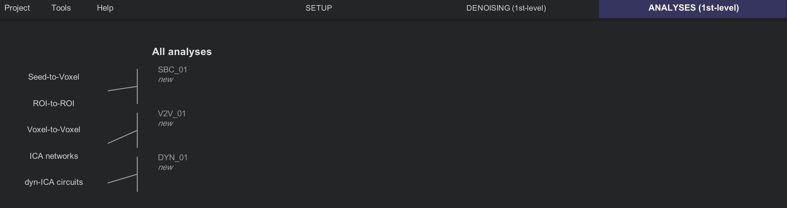
The 1st-level tab. Seed-to-voxel and ROI-to-ROI analyses will be stored in a folder called SBC (Seed-Based Correlation), Voxel-to-Voxel analyses will be stored in the folder V2V (Voxel-to-Voxel), and dyn-ICA circuits will be output in the folder DYN_01 (Dynamic Connectivity).
Seed-Based Correlation
If you recall from the Setup tab, several different ROIs were generated: Grey matter, white matter, and CSF (the latter two primarily for denoising using AnatCompCor), and atlases and networks. The atlases and networks ROIs parcellate the brain into different regions, also known as seeds. In each of the seeds the time-series of the grey matter is averaged across all of the voxels, and correlation maps are generated for both the correlation of that seed to all of the other seeds, and of each seed to all of the other voxels in the brain.
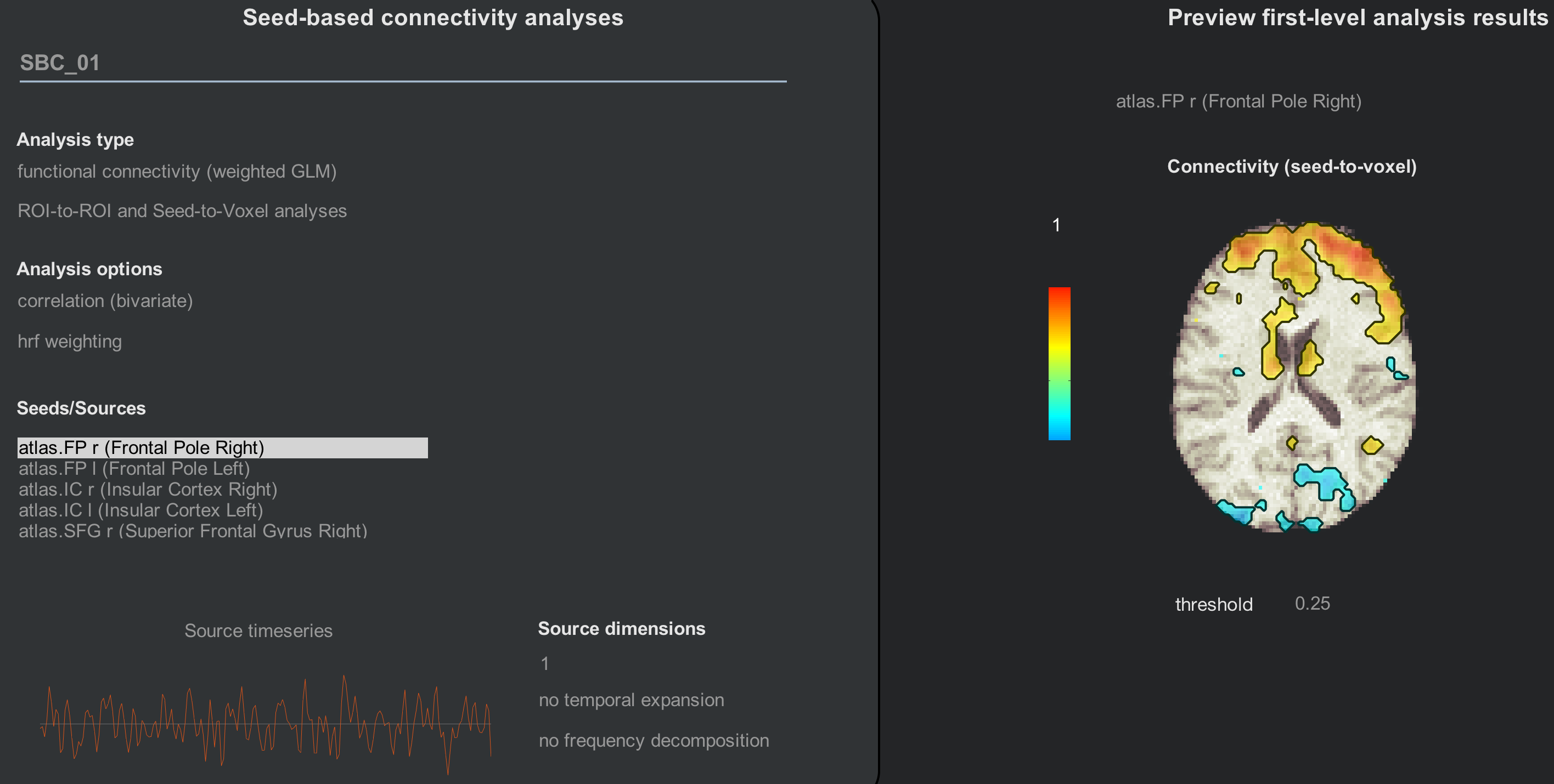
Clicking on the Seed-to-Voxel or ROI-to-ROI buttons (which are yoked together) will display two distinct areas, similar to the setup in the Denoising tab. The left area, Seed-based connectivity analyses, lists different analysis types and options that you can choose from. The right area, Preview first-level analysis results, shows how the averaged time-series of the currently selected seed correlates with other voxels in the brain.
Since we are only looking at resting-state data, functional connectivity (weighted GLM) is the most appropriate option to use. Later on we will see how to do a generalized psychophysiological interaction (gPPI) analysis, which can be used with task-related datasets.
In the Seeds/Sources panel, highlight different seeds to observe how the connectivity map changes in the Preview first-level analysis results area. What do you notice about the maps as you select different seeds? Do they match up with what you would predict?
If you are satisfied with the preview of the correlation maps, click the Done button. This will generate correlation maps that are stored in your project folder in the results/firstlevel directory. Once we have done this for all of the subjects in our dataset we can then run a group analysis, which we now turn to.
Video
To see how to do a 1st-level analysis on your computer, click here.